Introduction Link to heading
This project is my solution to the Handwritten to Data
Kaggle competition for Ukrainian handwriting recognition. Its dataset is publicly
available on Hugging Face as UkrainianCatholicUniversity/rukopys.
Part of my day job is on the deployment side of ML — porting and optimizing models to run on mobile phones, where the recurring questions are “does this fit in memory?”, “does it hit the latency budget?”, and “does it run on the target hardware?”. Within that, I work mostly on document AI: page detection, document classification, image enhancement. Handwritten-text recognition, though, was a piece of the stack I had never built end-to-end myself. I treated this dataset as a chance to fill that gap while staying inside the constraints I optimize for at work.
I also wanted to keep the project compact for a learning reason: small enough to retrain on a single machine, simple enough to iterate on quickly, and easy enough to debug that each new idea could be understood before the next one landed on top. Fine-tuning a heavyweight checkpoint would have hidden exactly the parts I wanted to learn.
The compact framing also matches a real production reality. Modern VLMs read handwriting impressively well, and when a high-end GPU is available at inference time, calling one is often the right move. But many deployment targets do not look like that. The serving box may be a CPU instance with no GPU at all, on-device inference may be a hard requirement, latency budgets may rule out multi-billion-parameter models per request, or a fast first-pass transcription may be refined by a heavier model downstream. For those settings, a compact classical pipeline is still the right starting point — not as a replacement for VLMs, but as the layer underneath or in front of them.
The end result is a ~36 MB (fp16) CPU-runnable pipeline that scores 0.811 on the competition metric — small enough to fit on a phone, transparent enough that errors can be traced to a specific stage, trainable by one person on one machine, and accurate enough to be useful as a first-pass transcription before any VLM refinement.
This article follows that path through the whole system: line detection, recognition, decoding, language-model rescoring, and the post-processing attempts that did not work. The interesting part is not a single model checkpoint, but the way each stage changes the error profile of the next one.
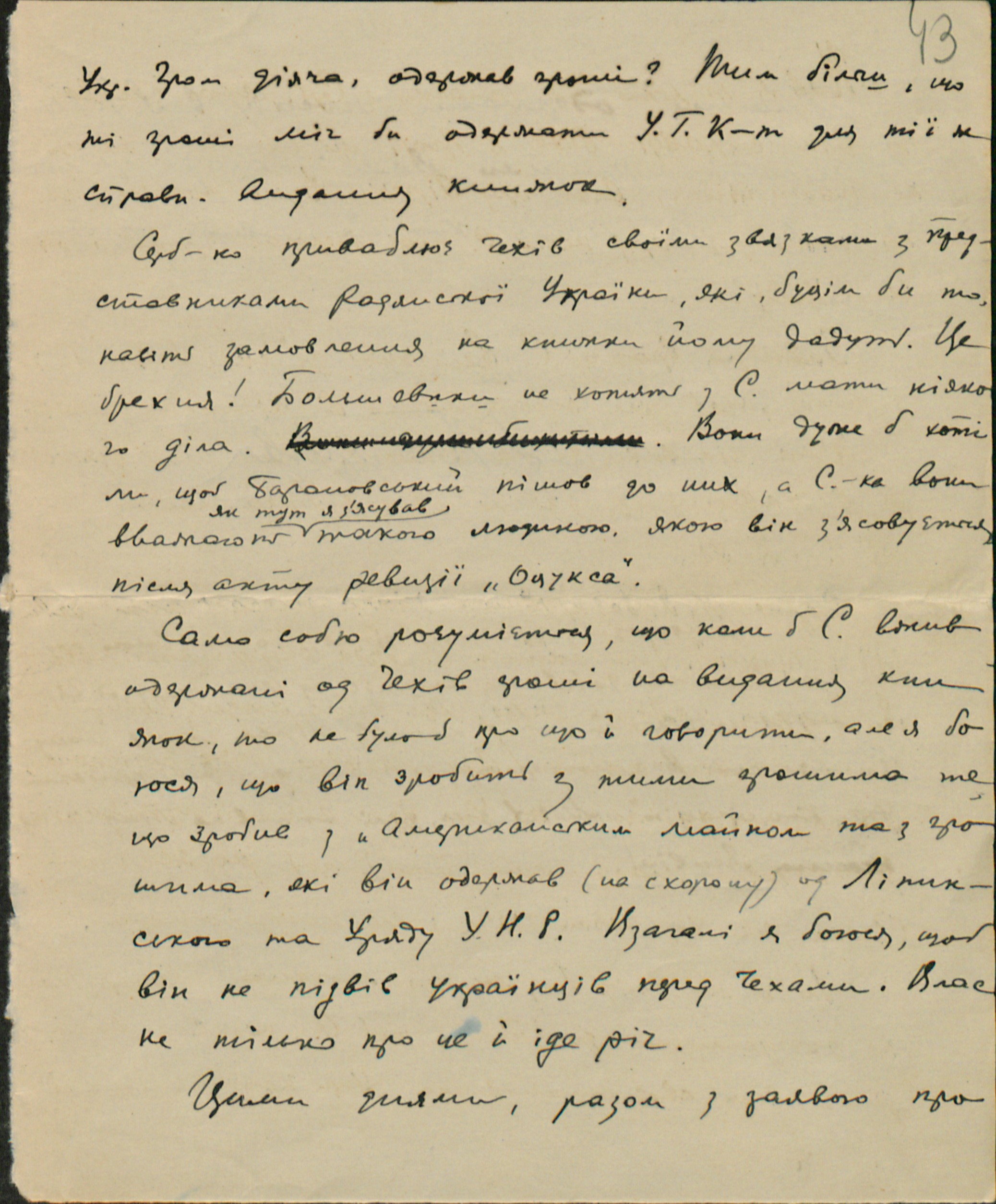
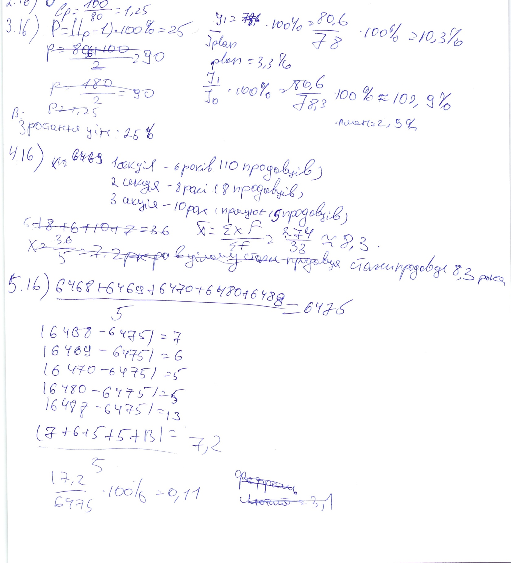
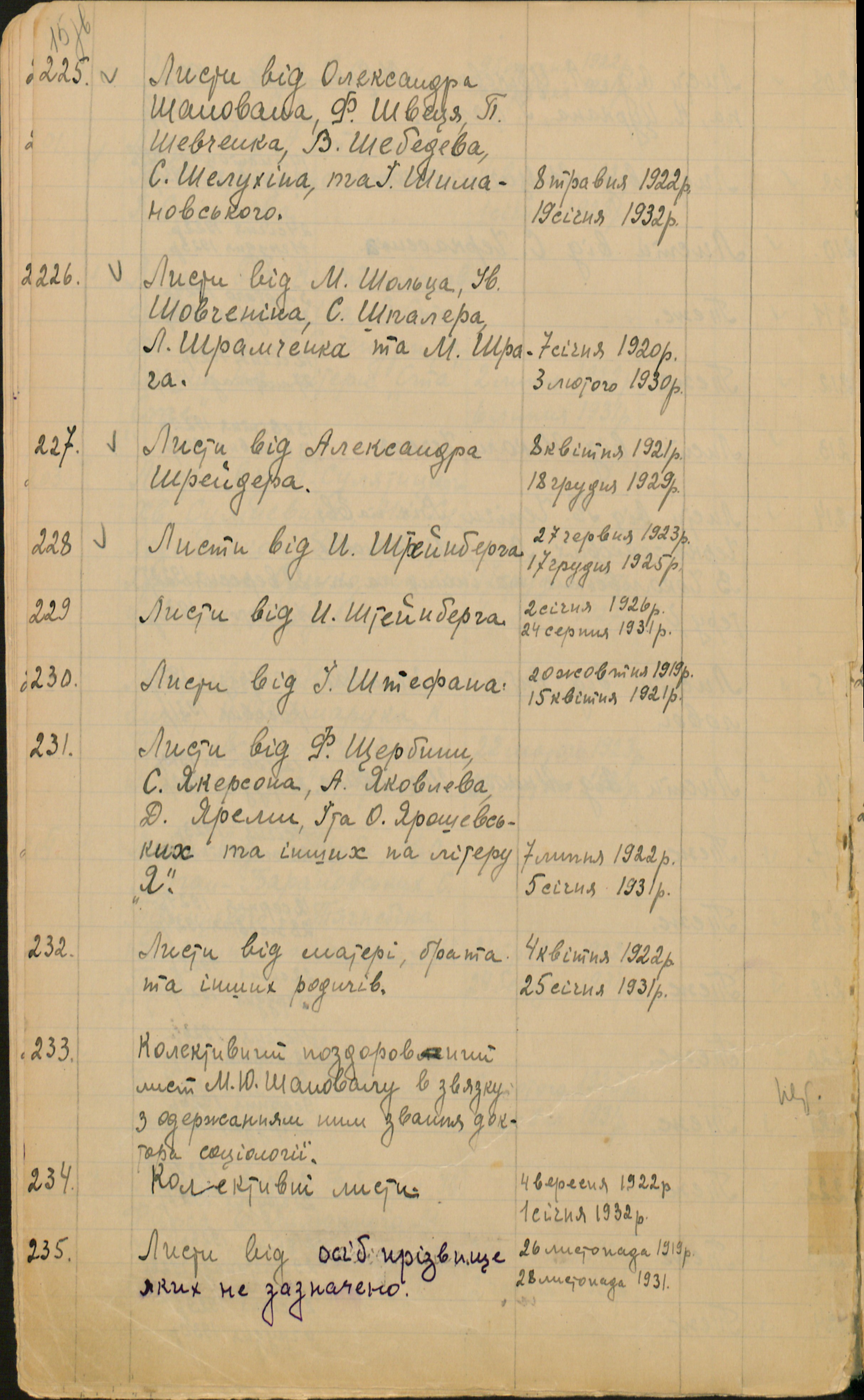
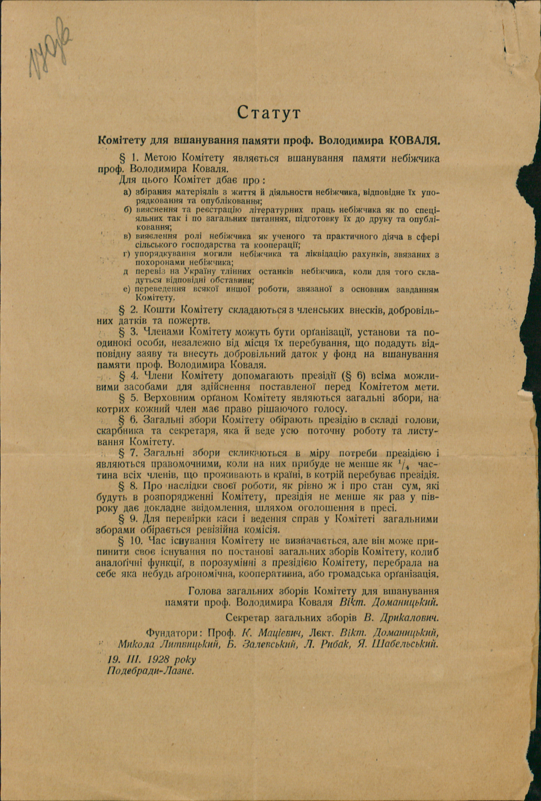
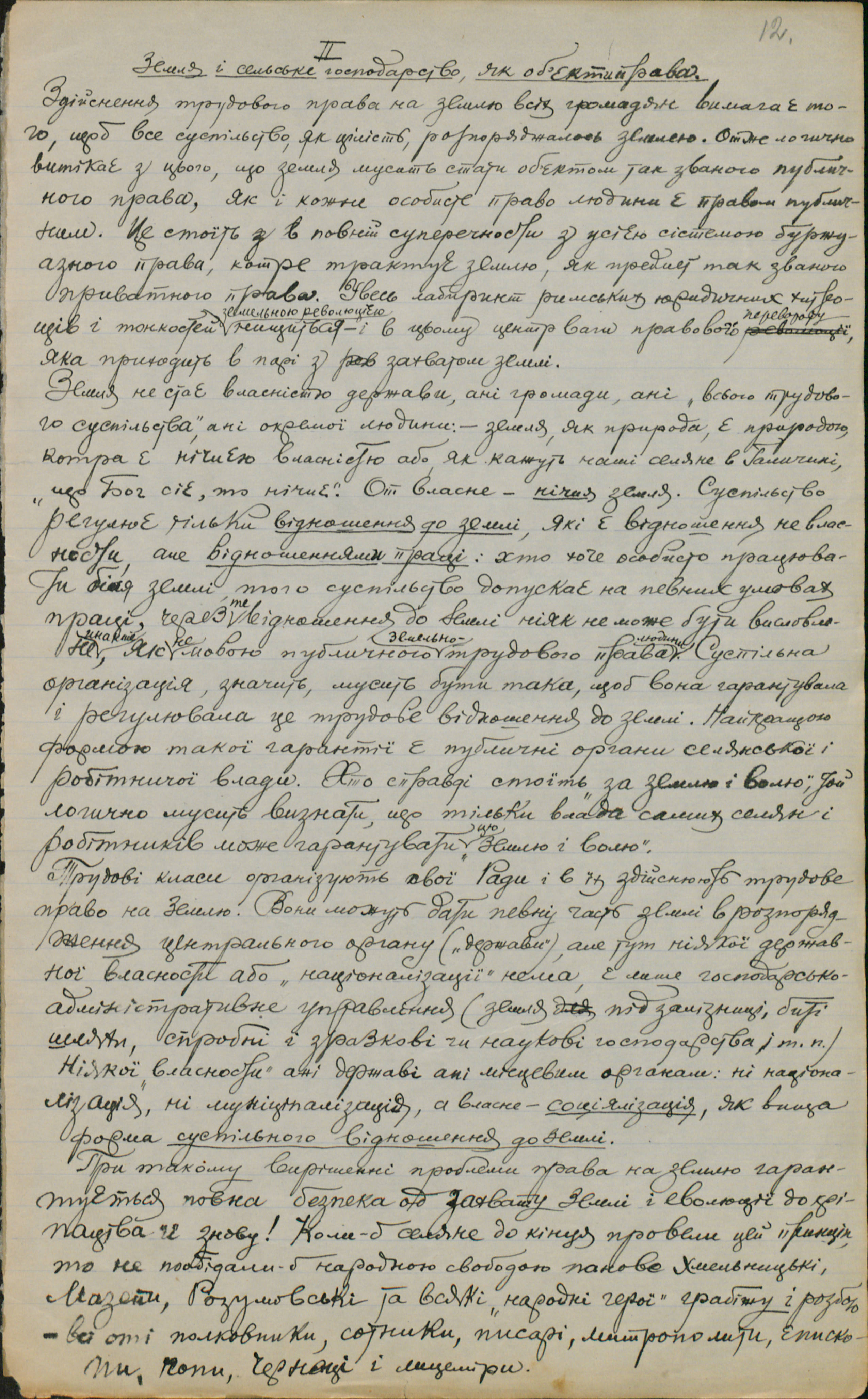
The dataset contains full-page handwritten documents and extracted recognition crops with different levels of difficulty: clean lines, dense pages, noisy regions, and ambiguous crops. A few examples are enough to show why this is a pipeline problem rather than only a recognizer problem.
Evaluation Metric Link to heading
The competition score was defined as:
$$ \begin{aligned} \text{Score} ={} & 0.15 \times \text{Detection F1} \ & + 0.05 \times \text{ClassAcc} \ & + 0.30 \times (1 - \text{CER}) \ & + 0.50 \times (1 - \text{PageCER}) \end{aligned} $$
The score is a weighted combination of detection, classification, and text recognition quality:
- Detection F1 (15%) measures type-agnostic bounding-box detection. A
predicted box counts as a true positive when its IoU with a ground-truth box
is at least
0.5. - Classification Accuracy (5%) is computed on IoU-matched region pairs and checks whether the predicted region type matches the ground-truth type. Region types include handwritten, printed, formula, table, annotation, image, and graph.
- Character Error Rate (30%) is computed per region and averaged over
scorable regions. A region is scorable when the ground truth has
language=uk,legibility=legible, and the type is notimageorgraph. - Page CER (50%) compares full-page text. Ground-truth and predicted regions are sorted by reading order, concatenated into strings, and compared with Levenshtein distance. This component is agnostic to box granularity and rewards correct page text even when individual boundaries are not perfect.
1. Line Detection Link to heading
Framing the Detection Task Link to heading
The first step was to look at the available annotations and decide how to formulate the detection problem. Since the dataset already provided text-line bounding boxes, the most obvious starting point was a YOLO-style detector.
This approach has several practical advantages:
- simple annotation format;
- mature training and evaluation pipelines;
- fast inference;
- rather small models.
However, handwritten text lines are not natural rectangular objects. They are long, thin structures that may be curved, densely packed, and separated by only a few pixels. Representing them with bounding boxes introduces several challenges:
- Dense pages produce many overlapping boxes, making non-maximum suppression an important part of the detection pipeline.
- Curved or slanted lines are only approximated by rectangular regions.
- Neighboring lines can touch or overlap vertically, making box boundaries ambiguous.
- A correctly localized box does not necessarily produce a good recognition crop.
- Bounding boxes describe where a line is located, but provide little information about how adjacent lines should be separated.
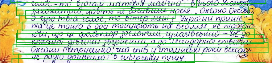


These observations suggested that the task might be better formulated as a segmentation problem rather than a pure object-detection problem. Instead of predicting a rectangle around each line, the model could predict the geometric structure of the page and leave the final line extraction to a dedicated postprocessing stage.
ARUNet Link to heading
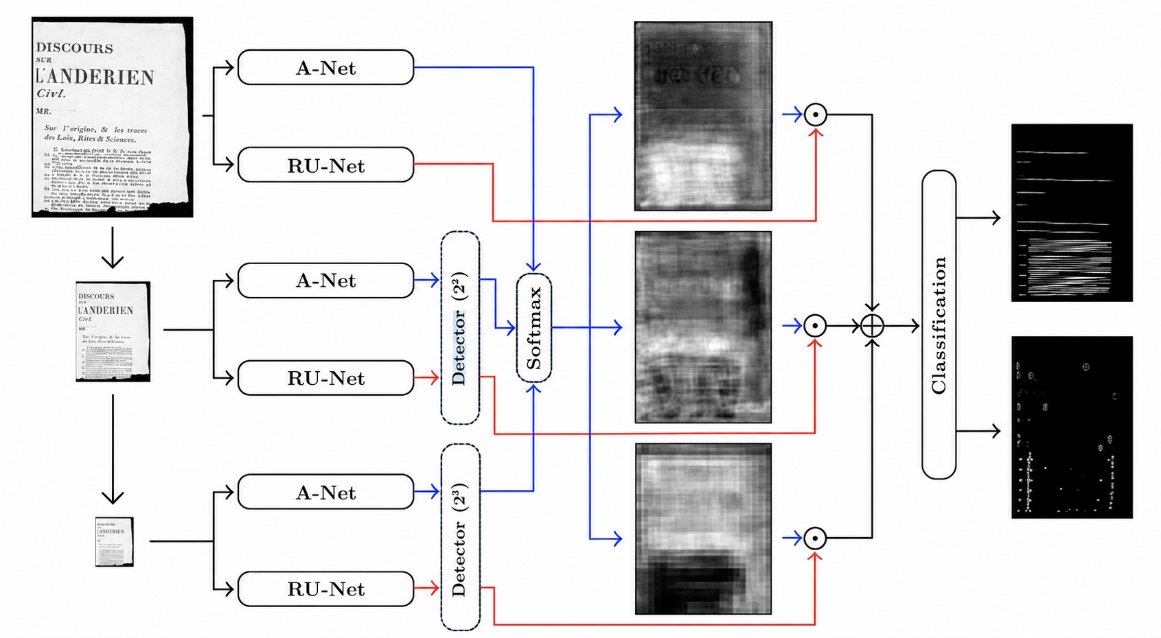
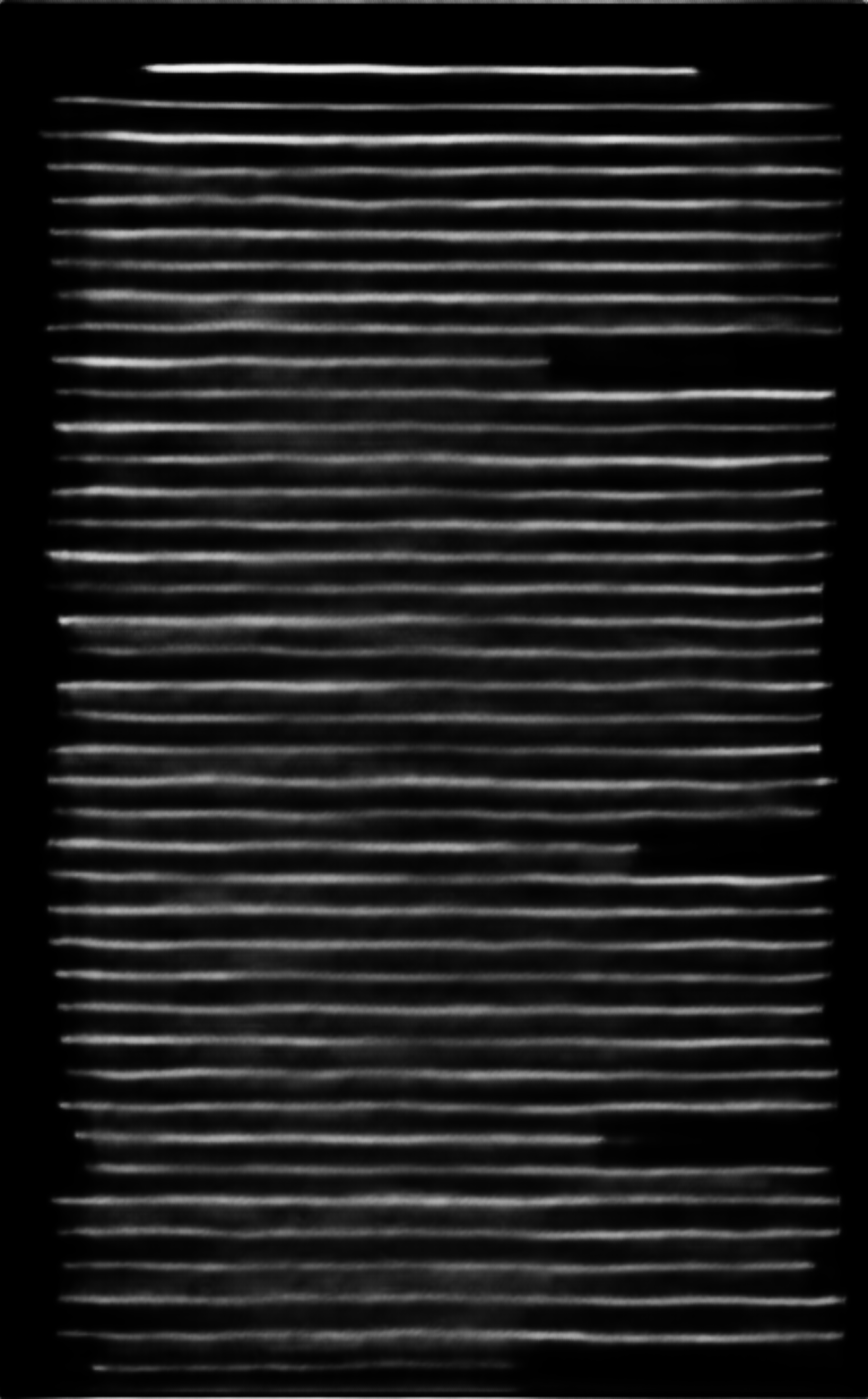
For line detection I used an ARUNet-style segmentation model from A Two-Stage Method for Text Line Detection in Historical Documents. Instead of predicting boxes, it produces dense centerline and separator maps, which handle curved text, touching lines, and variable spacing more explicitly. Conceptually, it is a U-Net encoder-decoder network with attention blocks added to improve spatial focus. The encoder extracts increasingly abstract page features, while the decoder upsamples them back to pixel-level prediction maps.
The important part is that the model remains fully convolutional: it predicts dense maps over the whole page instead of proposing individual boxes. Spatial attention helps the decoder focus on relevant text-line structures while suppressing background texture, page noise, and unrelated strokes.
The training targets are not rectangular boxes. They are dense supervision maps: one map describes likely text centerlines, and another describes separator regions. Given the original bbox annotations, I rasterize the supervision maps from the box geometry itself: the box centerline defines the positive centerline trace, and the box height determines how much vertical support belongs to the line versus the separator bands around it.
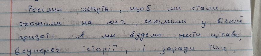
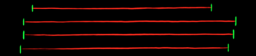
The line-probability map replaces rectangular proposals with a soft centerline signal, while the separator map gives postprocessing an explicit cue for splitting nearby text regions. This is the part that makes the method useful on dense pages where bounding boxes and connected components tend to become unstable.

Postprocessing: From Probability Maps to Lines Link to heading
The network output is not a set of text lines. It is only a pair of probability maps.
The centerline map answers: “where is the middle of a text line likely to be?” The separator map answers: “where should neighboring text regions be kept apart?”
Those maps are useful, but the recognizer needs something more concrete: ordered line crops. Each crop should contain one target line, preserve ascenders and descenders, and avoid leaking text from nearby lines.
This is where postprocessing becomes a real part of the OCR system rather than a small cleanup step. I partially followed the logic from A Two-Stage Method for Text Line Detection in Historical Documents: use the neural network to produce soft geometric evidence, then use classical image-processing and graph logic to recover line instances.
Sparse Line Points Link to heading
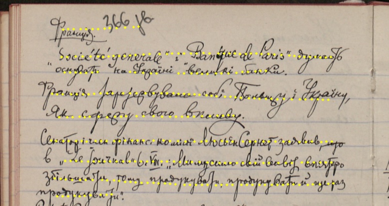
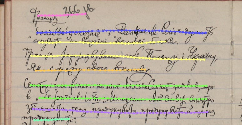
The first step is to reduce the dense centerline map to a sparse set of points. The map is thresholded, skeletonized, and sampled into representative points on likely text centerlines. This keeps the postprocessor lightweight: instead of reasoning over every pixel, it reasons over a compact set of line points.
Graph Linking Link to heading
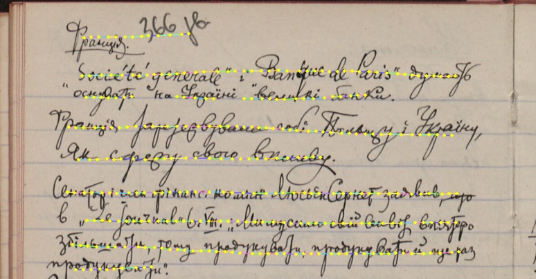
The next step links nearby points that plausibly belong to the same text line. The links use local direction, spacing, and centerline confidence, while the separator map discourages connections across neighboring lines. In code, the candidate edge score is a weighted sum of forward distance, perpendicular offset, orientation mismatch, and a long-offset penalty, with hard filters on angle, gap size, and intervening candidates. The result is a sparse graph where edges mean: “these points probably continue the same line.”
Line Fragments and Merging Link to heading
Connected components of the graph become initial line fragments. These fragments are intentionally conservative: faint ink, gaps in the centerline map, or ambiguous spacing can split one real text line into several pieces. A merge step then joins fragments when their geometry and centerline support are consistent.
Recognition Boxes Link to heading
The final recognizer cannot read a one-pixel centerline. It needs an image crop containing the full handwriting around that line. The last step therefore converts merged line fragments into recognition boxes, then expands them enough to keep ascenders, descenders, and small baseline errors inside the crop.
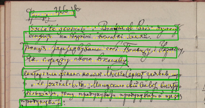
This last step is where detection becomes directly tied to recognition quality. A crop that is too tight loses strokes. A crop that is too large introduces text from adjacent lines. The postprocessor has to find a practical middle point, and doing it explicitly makes failures inspectable.
The result of this postprocessing is a list of ordered recognition crops. This style was useful because it kept the neural network output simple while making the conversion from dense maps to line crops inspectable. It also made failures easy to categorize: missing centerline evidence, wrong links, broken fragments, or boxes that include too much neighboring text.
What graph-based postprocessing gives you in practice:
- explicit, inspectable control over how nearby lines are split, via the separator map;
- line recovery from sparse evidence — broken or faint centerlines can still be linked into a coherent line;
- intermediate stages (sparse points → links → fragments → boxes) that can be visualized and inspected separately;
- recognition crops that can be evaluated independently of the recognizer.
2. Recognition Link to heading
Baseline: CRNN + CTC Link to heading
After the detector started producing usable line crops, the next question was recognition. For the first baseline I wanted something deliberately simple: a model that is easy to train, easy to debug, and fast enough to run locally.
I used the setup described in Best Practices for a Handwritten Text Recognition System as the starting point: a CRNN-style recognizer trained with Connectionist Temporal Classification. The point was not to build the strongest possible recognizer immediately, but to create a stable baseline that could tell whether the line detector was good enough.
The baseline recognizer has three main parts:
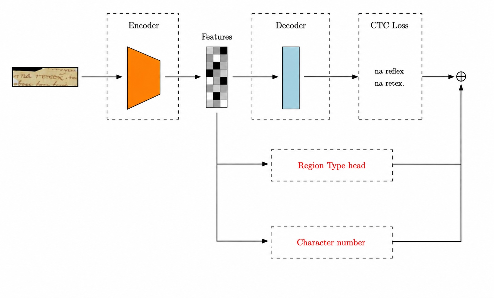
The recognizer includes a small spatial transformer block from the start. It learns a lightweight affine correction before feature extraction, which helps normalize slanted or slightly shifted line crops without a manual perspective step.
The CNN extracts visual features from the normalized line crop. The feature map is converted into a left-to-right sequence, the BiLSTM models context along the line, and a small time-axis self-attention block with 4 heads can refine the sequence before the final CTC classifier predicts character probabilities for each time step.
CTC is a natural fit here because the training data gives the final text string, not character-level positions. The model is allowed to learn the alignment between image columns and output characters by itself:
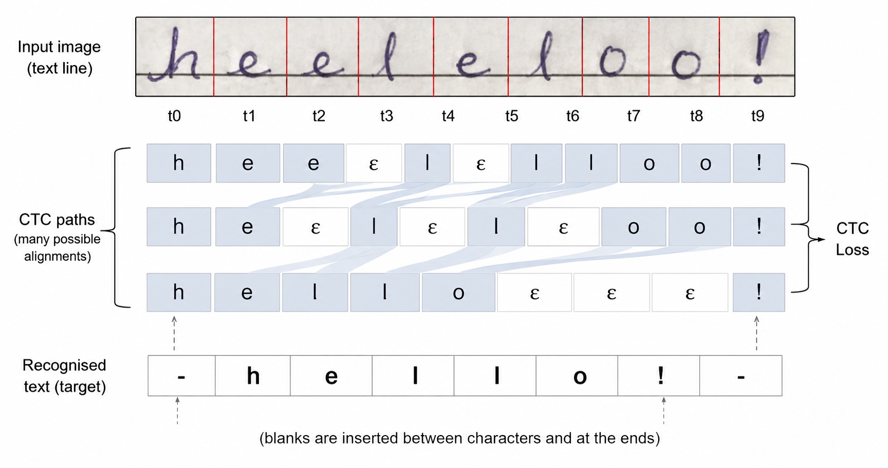
This makes the recognizer much easier to train than a fully supervised character-segmentation model.
The preprocessing step matters as much as the model:
- Recognition crops are resized to
128 x 1024(height x width). Smaller crops keep their aspect ratio and are padded, while larger crops are resized to fit. - During training, I apply on-the-fly geometric distortions and intensity perturbations as light handwritten-text augmentation.
- To match the padding around the image, the target text is extended with a boundary space token before and after the actual transcription. This avoids forcing the first and last characters to align directly with the crop boundaries.
I added two small auxiliary branches around this baseline:
- Auxiliary CTC shortcut head. A convolution-only branch trained with its own CTC loss. It projects directly to the character vocabulary and helps optimization by giving the encoder a shorter gradient path, in the same spirit as a residual shortcut.
- Region-type head. A classifier for handwritten text, printed text, formula, annotation, and other region classes used in the dataset. It does not transcribe text directly, but it gives a useful diagnostic signal when one content type fails much more often than others.
This was a good first recognizer because it was stable, fast, and easy to debug. If it failed on clean crops, the recognition model was likely the problem. If it worked on clean crops but failed in the full pipeline, the detector or crop postprocessing was more likely responsible.
Problem: Printed Text Recognition Failures Link to heading
The first serious debugging loop started with printed text. Based on visual inspection, these lines looked easier than handwriting: the glyphs were clean, the spacing was regular, and the crops were usually readable. But the validation metrics showed many errors for printed regions.
At first this looked suspicious. If the model fails on messy handwriting, there are many possible explanations: bad crops, ambiguous letters, inconsistent labels, or weak language modeling. But when it fails on clean printed text and produces complete nonsense, the problem is often more structural.

After more inspection, the problem turned out to be structural.
Before CTC classification, the CNN encoder converts the crop into a left-to-right
feature sequence. Its convolution and pooling layers reduce the horizontal
dimension to make recognition cheaper. In the original encoder, the cumulative
horizontal reduction was about 16x: a crop with useful width W produced only
about W / 16 CTC timesteps. A compact printed line can therefore be visually
clear but still leave the CTC head with too few positions for its characters.
CTC needs enough input steps to align the output string. It is not enough that the image is readable to a human. The model needs a time dimension long enough to place characters, repeated characters, and blanks.
Printed text is denser than handwriting, so the same crop width can contain many more characters. I measured this with a simple ratio:
1ctc_ratio = sequence_length / label_length
Low-ratio samples were the failures to inspect first. If the sequence is shorter than the label, alignment is impossible; even slightly above that threshold, CTC has little room for blanks and repeated characters.
The W in this calculation is the crop width after aspect-preserving resize,
not the full padded 1024-pixel canvas. Padding fills the remaining canvas but
does not create useful visual timesteps. The target length also includes one
boundary space before and after the transcription, so the plotted label length
is the visible text plus two CTC tokens. With 16x horizontal downsampling,
every point below the diagonal has fewer usable timesteps than target characters
and therefore cannot be aligned by CTC.
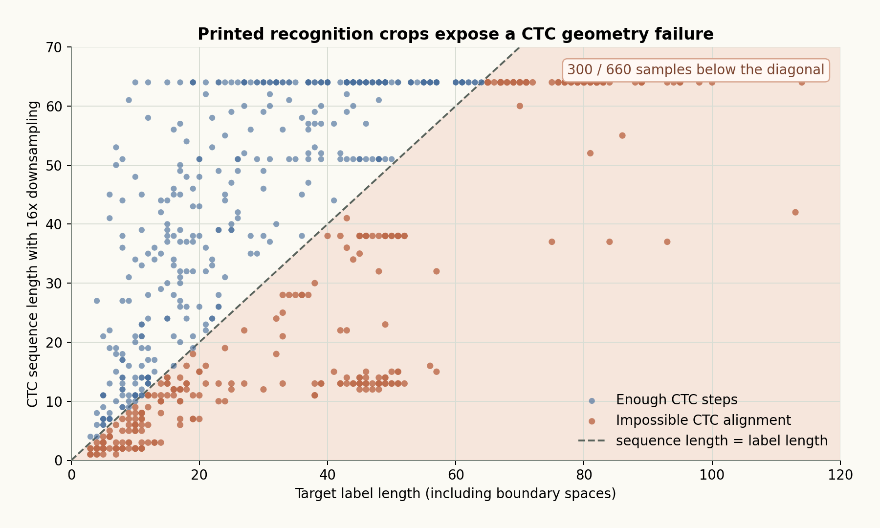
Sorting by this ratio matched the manual failures: clear printed crops with long
labels and too few CTC timesteps. The fix was to change the first convolution’s
horizontal stride from 2 to 1. This reduced the encoder’s cumulative
horizontal downsampling from 16x to 8x, doubling the number of CTC
positions available for the same crop without changing the recognizer interface.
Dataset Cleaning Link to heading
The next issue was not architectural. It was data quality.
For OCR datasets, it is easy to assume that the labels are correct because they came from an annotation pipeline. In practice, this assumption is dangerous. A recognizer trained on noisy labels can look like a weak model even when the architecture is fine.
I treated this as an active-learning cleanup problem:
1Train baseline recognizer
2    ↓
3Evaluate training samples
4    ↓
5Find suspicious samples by metrics
6    ↓
7Inspect and clean labels/crops
8    ↓
9Retrain recognizer
The idea is simple: once the model is good enough, its largest training-set errors are often not “hard examples” anymore. Many of them are annotation problems, broken crops, or samples whose image does not match the target text.
For the check step, I used several metrics:
- CER: normalized character error rate between prediction and label.
- Prediction confidence: low-confidence predictions are useful candidates for inspection.
- Region-type classifier confidence: high-confidence disagreement between expected and predicted type can reveal mislabeled regions.
The main filters were:
- high
CER; - high classifier confidence for a different region type;
- low recognizer confidence combined with a large text mismatch.
After sorting candidates by those signals and opening the images manually, several problems became obvious.
Some crops contained more than one text line. In those cases the model had no principled way to know which line the label referred to. The image might contain two readable lines, while the target contains only one of them:
1crop image:  line A + line B
2target:      line A
3model:       line B, or a mixture of both
Those samples are especially harmful because the visual input and label are both valid text, but they do not describe the same recognition task.

This is particularly bad for CTC training: if the crop contains two lines, there is no single left-to-right target sequence, so the network can align the wrong line and learn noisy supervision. Removing these multiline samples made the training objective more consistent.
Other crops were simply messy: partial words, broken extraction, wrong region boundaries, or fragments where even a human would need surrounding context. Keeping those samples in training teaches the model inconsistent alignments.

I also used the classifier head to find region-type mismatches. For example, if a crop is labeled as handwritten but the classifier is highly confident that it is printed or formula-like, that sample becomes a review candidate.
The important part is that removal was not fully automatic. Metrics were used to rank suspicious samples, then the final decision was made by visual inspection. Multiline crops, broken crops, and clear wrong-label examples were moved out of the training set. After cleanup, the recognizer was trained again on the refined dataset.
Result after cleanup:
1ARUNet + CRNN + greedy CTC: 0.746
3. Detection Improvements Link to heading
Detection Was Still the Bottleneck Link to heading
After the first end-to-end version, the result was useful but the error analysis pointed back to detection. The recognition model was already sensitive to crop quality: if a crop contained extra text from a neighboring line, or if the target line was cut too tightly, the recognizer could fail even when the text itself was readable.
Many pages were easy. When the lines were straight, well separated, and close to horizontal, the graph-based postprocessor produced good crops. These are the cases where the recognizer receives a clean line image and can do its job.

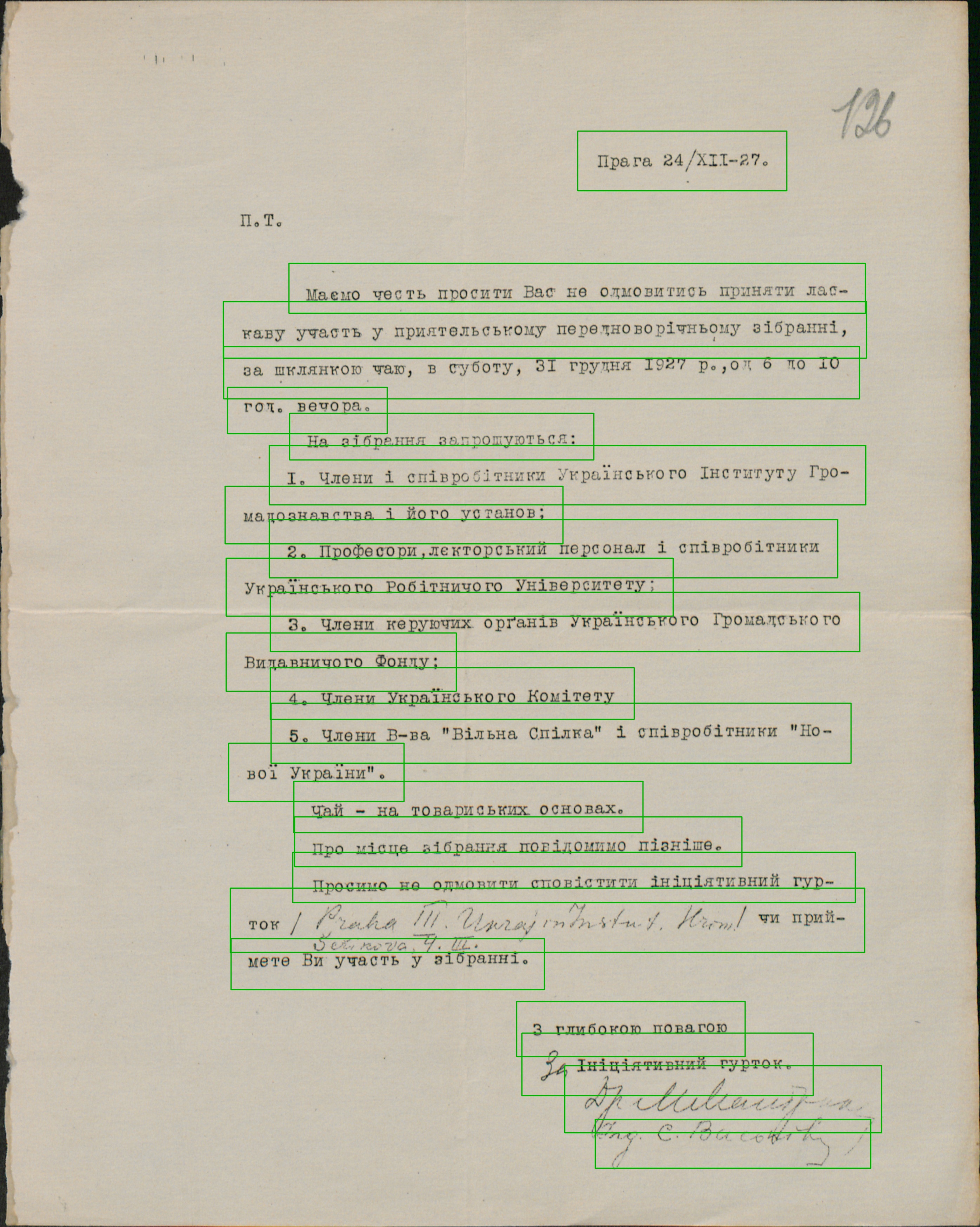
But the dataset also contained harder layouts:
- pages with separated blocks of text;
- curved baselines;
- text written under a noticeable angle;
- dense regions where neighboring lines were close;
- crops where a small amount of extra text changed the recognizer output.
The difficult cases were not always dramatic. Sometimes the oriented box looked reasonable, but the crop still included part of the line above or below. For CTC recognition, this is enough to break the assumption that one crop corresponds to one target sequence.
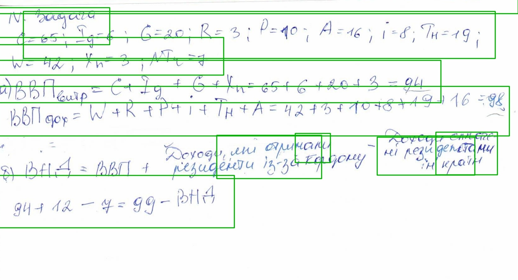
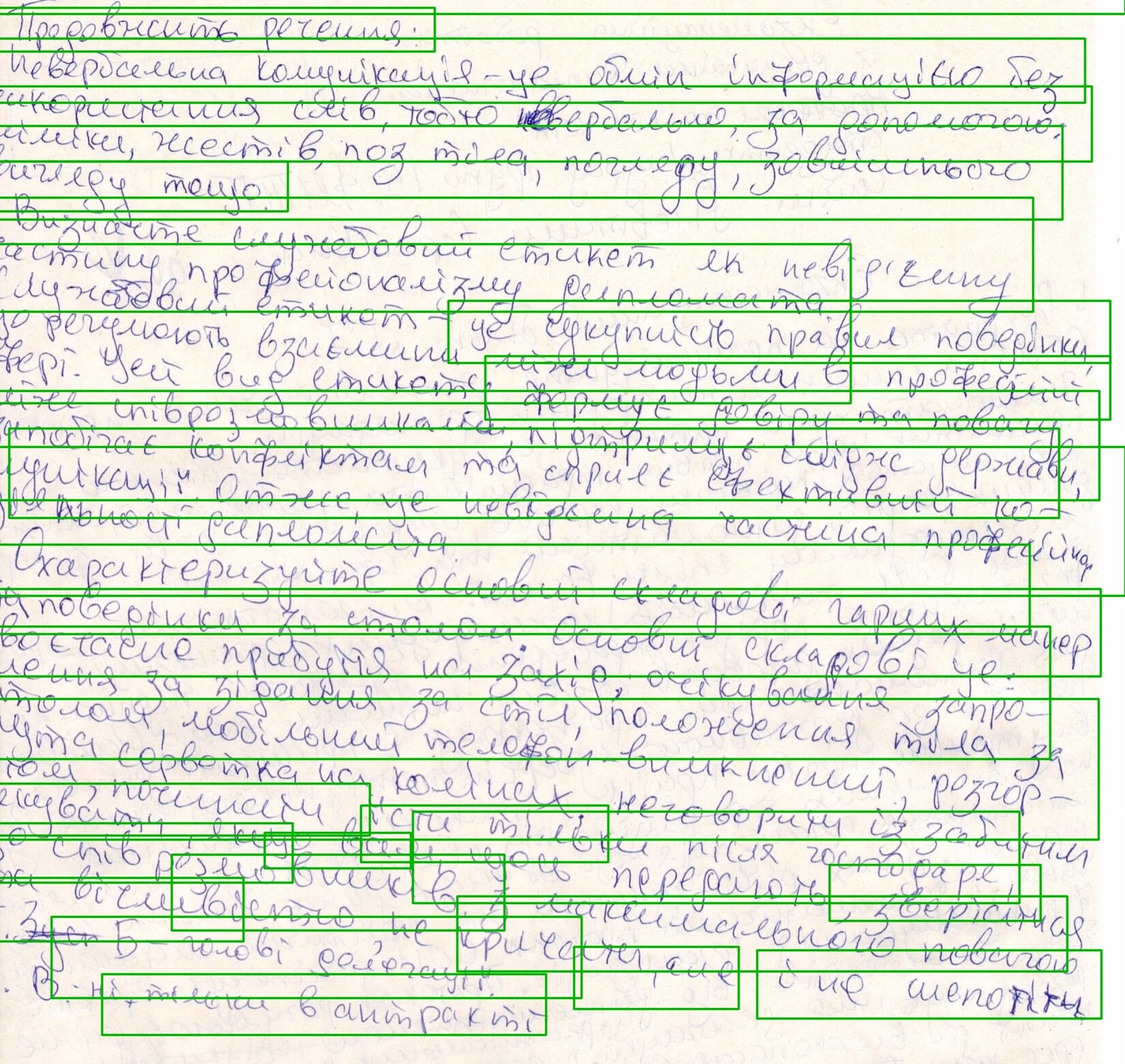
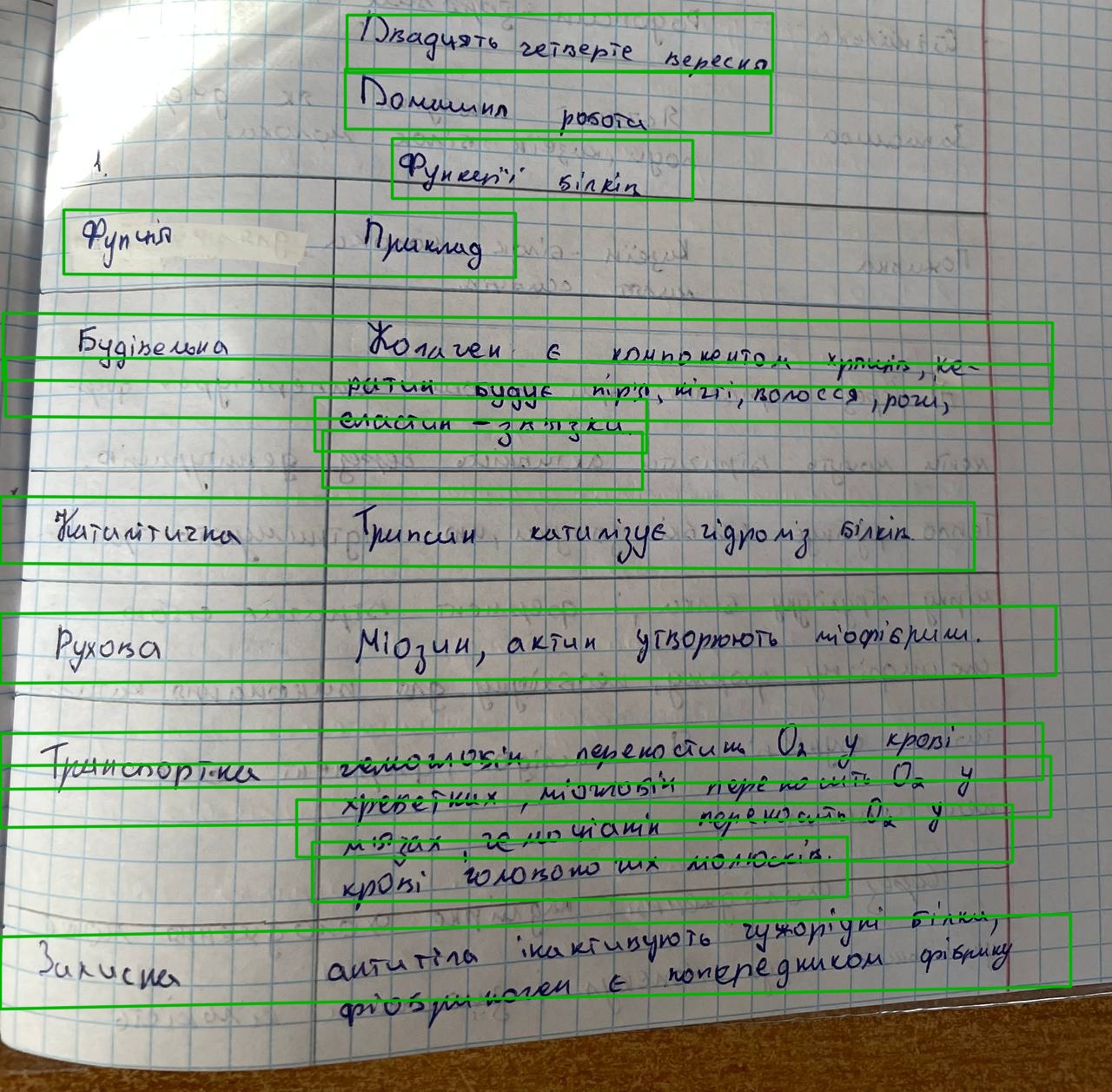
The conclusion was clear: improving recognition required improving detection. A better recognizer can tolerate some noise, but it cannot reliably choose the intended line when the crop contains multiple plausible text sequences.
Watershed Postprocessing Link to heading
The next postprocessing idea was to treat line extraction as an instance-segmentation problem. The network already predicts two useful maps:
- line probability: where text centerlines are likely to be;
- separator probability: where neighboring lines should be split.
The watershed postprocessor converts those maps into line instances. The idea is to create reliable markers from high-confidence line regions, restrict growth to a foreground band around line evidence, and use separator predictions as barriers between competing instances.
Step-by-Step Watershed Extraction Link to heading
1. Prepare the prediction maps. Very large maps are reduced to a bounded processing resolution. The line prediction is thresholded into a binary support map, and peaks in its row-wise density estimate the typical spacing between text lines on the page.
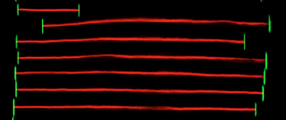
2. Build markers and the foreground band. High-confidence line pixels are horizontally closed, filtered, and merged when their endpoint geometry and bridge support agree. A lower threshold then creates the foreground band, dilated vertically using the estimated line spacing. The markers are the seeds; the foreground band limits where they may grow.
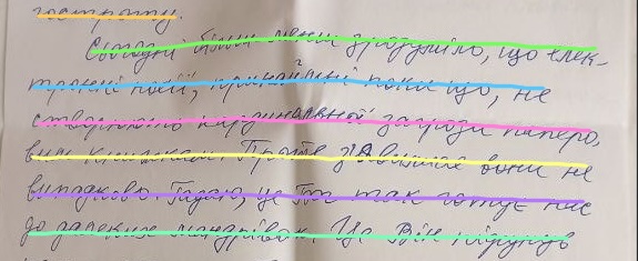
3. Grow, validate, and expand line instances. Watershed uses the elevation 1 - line_support + 0.2 * separator_probability, so separator predictions act as barriers between neighboring lines. Tiny, narrow, and border-only regions are removed. Separator components near baseline endpoints estimate crop height, then the remaining masks expand competitively into the final recognition regions.
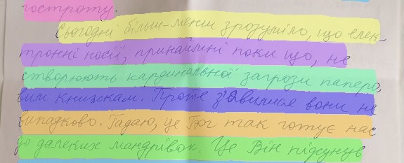
The separator map is important in two places. First, it raises the watershed elevation, making it harder for neighboring line instances to cross separator regions. Second, separator components help estimate line height near baseline endpoints. That gives better crops than relying only on a global line-spacing heuristic.
Compared with graph-based connected components, watershed gives a denser interpretation of the page. Instead of starting from sparse superpixels and linking them into curves, it creates competing regions in image space. This is a better fit when line geometry is not cleanly represented by a small set of connected baseline points.
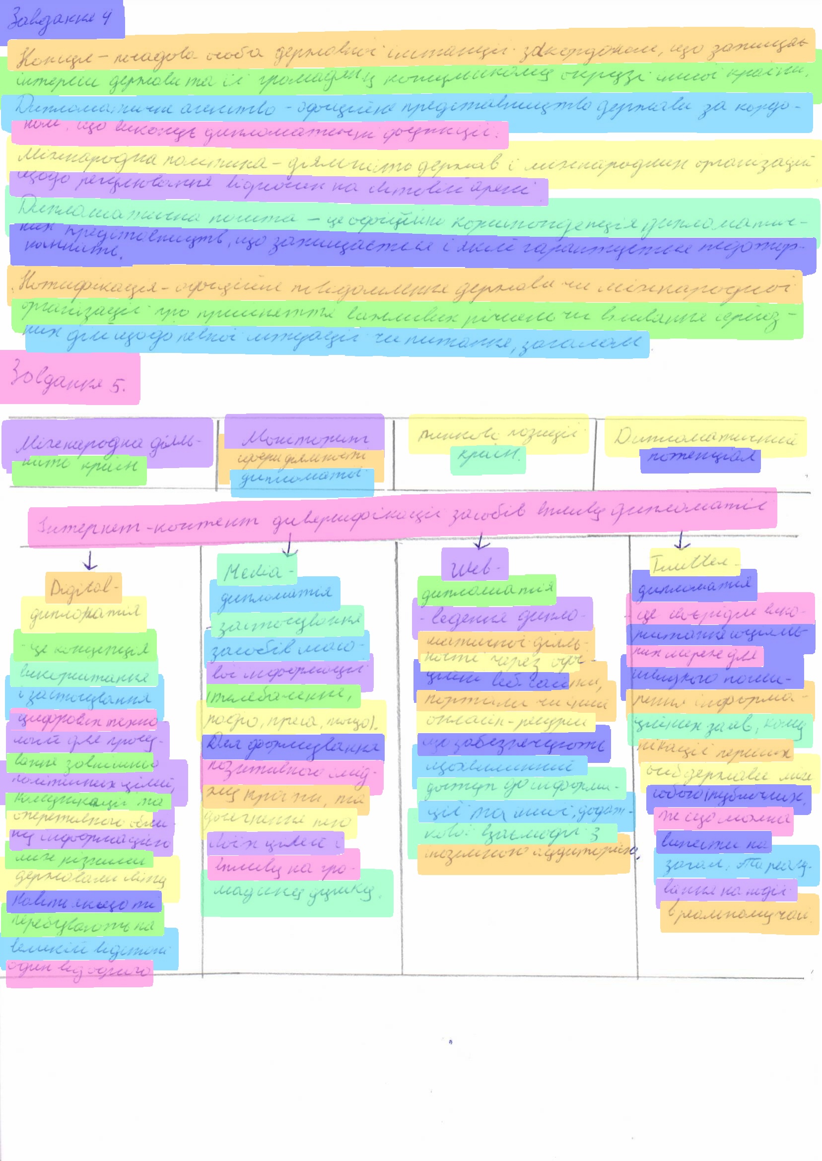
An important follow-up idea was to stop treating the oriented box as the final recognition object. Once watershed gives an instance mask, the crop does not have to be a pure rectangle anymore. This changes the problem. The bbox is only a container used to extract pixels from the page. The mask decides which pixels belong to the line. Extra neighboring text can be suppressed before the recognizer sees the crop.


This is useful because recognition is sensitive to additional text. If a neighboring stroke is inside the rectangle but outside the instance mask, those pixels are filled with the mean crop color instead of being left as-is. I did not add a separate perspective transform at this stage; geometric normalization is handled inside the recognizer by the Spatial Transformer. The recognizer receives a cleaner visual sequence, while the detector keeps the more flexible geometry of the watershed instance.
The goal was not to make postprocessing more complex for its own sake. The goal was to reduce extra text in recognition crops, because recognition quality was already limited by crop purity.
Result after Watershed:
1Previous: 0.746
2ARUNet(watershed) + CRNN + greedy CTC: 0.771
4. Recognition Improvements Link to heading
Beam Search Decoding Link to heading
Even a strong recognizer produces uncertain outputs. Greedy CTC decoding takes the best character at each time step and then collapses repeats and blanks. It is fast, but it throws away useful alternatives. Beam search keeps several possible prefixes alive while scanning the CTC output, so the final decision can use more than only the locally best visual character.
That matters because the recognizer often produces ambiguous probabilities:
1visual crop -> CTC probabilities -> beam hypotheses
2                                  -> "земля"
3                                  -> "земла"
4                                  -> "земпя"
The visual model proposes several plausible readings. The decoder decides which one survives.
Character-Level RNN Language Model Link to heading
Using only visual information is a lightweight starting point and already gives usable initial results, but it ignores a simple fact: text has structure. Some character sequences are common, some are rare, and some are almost impossible in the target language or domain. Adding this linguistic information during decoding is a standard way to improve CTC-style recognizers. Similar ideas are used in joint CTC/attention speech recognition with an external RNN-LM (Advances in Joint CTC-Attention based End-to-End Speech Recognition with a Deep CNN Encoder and RNN-LM) and in OCR systems such as PyLaia (Improving Automatic Text Recognition with Language Models in the PyLaia Open-Source Library).
For this step I trained a small 2-layer LSTM language model. The training
corpus combined the original OCR texts with additional Ukrainian text mined
from the Internet. The validation perplexity ended up around 6.0, which was
good enough to provide a useful decoding prior without turning the LM into the
main source of prediction.
During decoding, the language model does not replace the recognizer. It only adds a score to each beam expansion:
1score(prefix + c) = CTC_prefix_score(prefix + c) + lambda_lm * log P_lm(c | prefix)
The decoder keeps an RNN hidden state for every active beam. When several beams need the next-character distribution, they are scored together in a batch, so the integration stays cheap. If the recognizer and the LM use slightly different character vocabularies, a small vocabulary mapping is used before adding the LM score.
The practical effect is modest but useful: the visual model still decides what is visible in the crop, while the language model nudges uncertain hypotheses toward more plausible text. It cannot fix a bad line crop or missing characters, and too much LM weight can make the decoder hallucinate common text. For this reason the LM weight is a decoding hyperparameter, not a hard correction rule.
Result after adding RNN-LM rescoring:
1Previous: 0.771
2ARUNet + CRNN + joined CTC/LM rescoring: 0.794
Beyond CRNN: Conformer Recognizer Link to heading
The CRNN baseline was useful, but it was not the end of the recognition story. Handwritten lines often need wider context: repeated shapes, long words, abbreviations, and characters that are only clear after looking at neighboring strokes.
So I replaced the recurrent sequence encoder with a Conformer-style recognizer, following Conformer: Convolution-augmented Transformer for Speech Recognition. The model still starts with CNN visual features, but the sequence is processed by Conformer encoder blocks. A 3-layer Transformer attention decoder sits on top:
 1line crop
 2    ↓
 3CNN visual features
 4    ↓
 5linear projection + positional encoding
 6    ↓
 7Conformer encoder blocks
 8    ↓
 9CTC head
10    ↓
11Transformer attention decoder
This gives two useful signals at the same time: self-attention for long-range dependencies and convolution for local stroke patterns. In practice, this is the right direction once the baseline recognizer is stable and the remaining errors are no longer only caused by bad crops.
Guided CTC Training Link to heading
Problem: CTC learns alignment slowly. It is efficient, but the alignment between visual timesteps and output characters is hidden during training.
Solution: use the idea from GTC: Guided Training of CTC Towards Efficient and Accurate Scene Text Recognition. The model uses one shared encoder with two heads: a CTC head for monotonic text prediction and an attention decoder head for sequence modeling. Training uses a weighted sum of the two losses, plus a small region-type classification term:
1L = 0.4 * L_ctc + 0.6 * L_attn + 0.1 * L_region
The attention head guides the shared encoder by backpropagating through the same trunk, so the CTC path learns alignment faster while the attention branch keeps sequence context available.
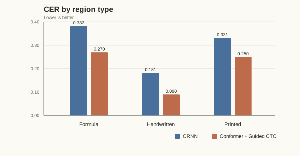
Result: the recognizer improved across categories. The baseline CRNN had
CER = 0.20, while the Conformer + Guided CTC model reached about
CER = 0.12.
Result after Conformer + Guided CTC:
1Previous: 0.794
2ARUNet + Conformer + Guided CTC: 0.804
Joint Attention, CTC, and LM Decoder Link to heading
The last step was to use all available scores during decoding. Instead of choosing only CTC or only attention, the beam decoder combines three signals:
- attention score: does the next character fit the output prefix?
- CTC prefix score: can it be aligned to the visual frames?
- RNN-LM score: is the character sequence plausible?
The combined score for extending a beam is:
1combined_delta = 0.6 * attention_delta + 0.4 * ctc_delta + 0.5 * lm_delta
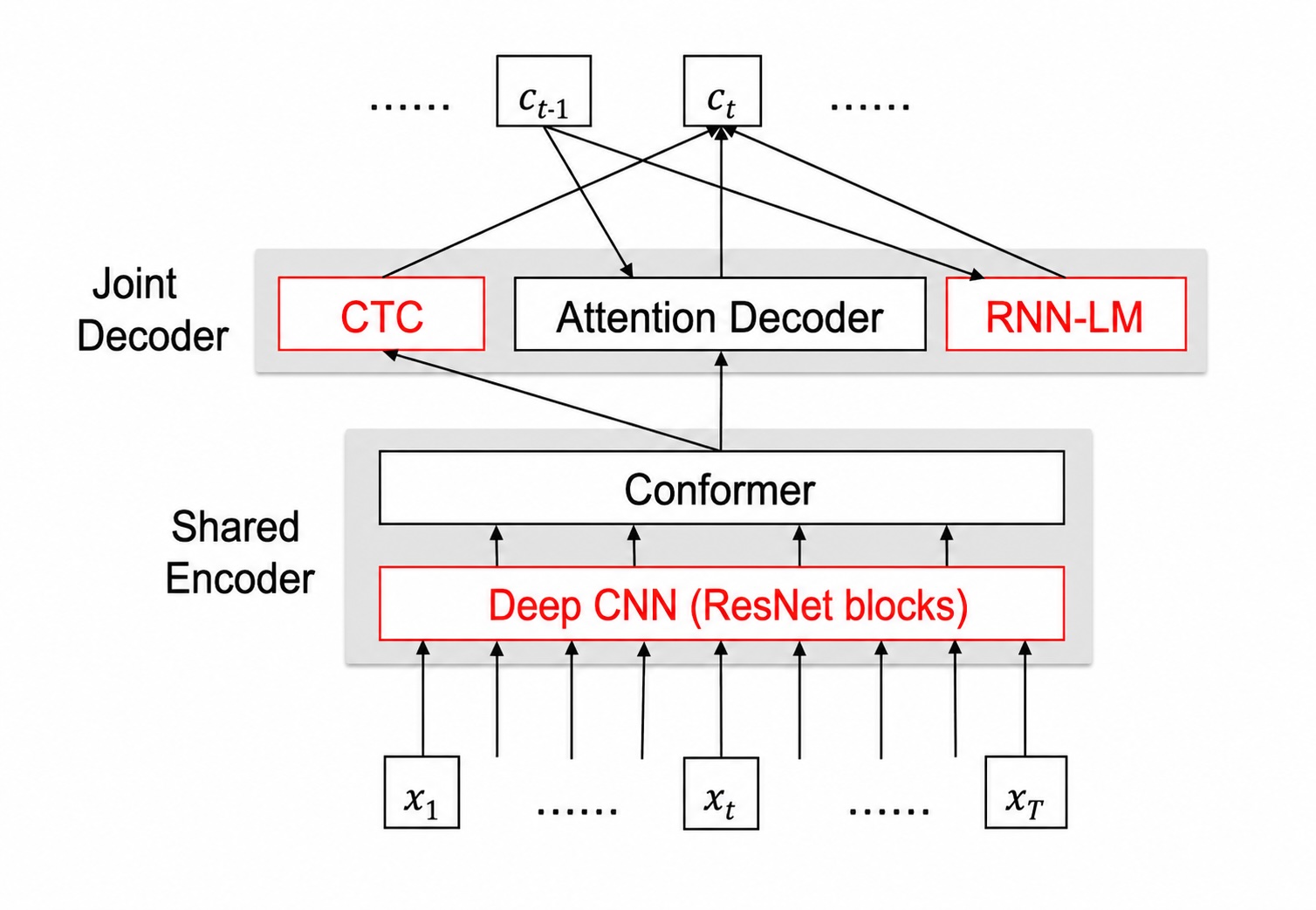
This decoder is more expensive than greedy CTC, but it is still only a line-level decoder. It does not solve document consistency, and it still cannot fix a bad crop. But for clean crops it reduces ambiguity: CTC anchors the output to the image, attention improves sequence modeling, and the language model nudges uncertain choices toward plausible text.
Together, the Conformer recognizer, guided CTC training, and joint Attention/CTC/LM decoding improved the final score further:
1Previous: 0.804
2ARUNet (watershed) + Conformer + Hybrid Decoder (CTC + Att + LM): 0.811
6. Remaining Failure Modes Link to heading
The final pipeline is much stronger than the baseline, but the remaining errors are still informative. They mainly come from ambiguous line instances and from recognition crops where visual evidence is genuinely weak.
Irregular and angled text. Even with better postprocessing, these layouts remain difficult. The baseline target is derived from the bbox centerline, which can be inaccurate for irregular lines, and the dataset contains relatively few such examples. A practical next step is to use a trained network to help relabel these pages and expand the training set with more complex cases.
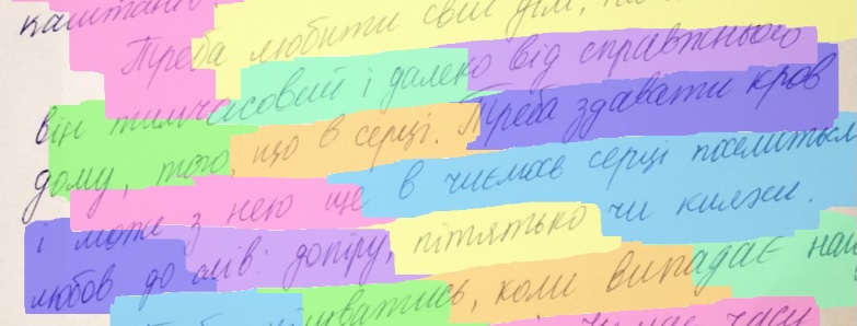
Difficult recognition crops. Some lines remain ambiguous even for a human reader. A useful next step is to include a small amount of surrounding document context and pass it with the OCR hypothesis to a vision-language model that can correct the transcription.

7. Negative Results Link to heading
Many OCR errors were small enough that the intended word still looked obvious. I explored several text-only post-processing approaches to correct them.
OCR Correction with Ranking.
1OCR token -> candidate words -> candidate ranking
This follows the candidate-generation + ranking shape that classical search and IR systems use:
- Candidate generation (SymSpell + beam search). SymSpell produced per-token dictionary candidates within a small edit distance, using a symmetric-delete index for fast lookup. A beam search then combined per-token candidates into whole-line corrections, keeping only the most promising prefixes.
- Ranking (bidirectional RNN-LM + priors). Two RNN language models — one running left-to-right, one right-to-left — scored each candidate line using context from both sides of every word. Frequency priors and edit-distance penalties kept the correction conservative.
The pipeline did not improve the final score consistently. The underlying assumption — that the correct word is a dictionary entry close to the observed token — does not hold for handwritten Ukrainian text. Historical spelling, names, and uncommon terms are valid out-of-vocabulary tokens, and the ranker could not separate them from genuine OCR errors. In practice, the correction stage sometimes replaced a correct OOV token with a more common but wrong one, so I left it out of the final pipeline.
CharacterBERT with CTC. A character-level BERT encoder with a CTC head maps noisy OCR lines directly to clean text. Self-attention lets each character use the whole line as context, while CTC can handle insertions, deletions, and length changes without a fixed character alignment. This should work when most of the phrase is clear and only a few words contain small OCR errors.
It did not improve the results. In many difficult examples, several words in the same phrase were corrupted, leaving too little reliable context for the model to infer the intended text. Ukrainian morphology also makes this a hard language-modeling problem for a small BERT trained on limited data.
WFST OCR Correction. A similar idea is described in Efficient OCR Post-Processing Combining Language, Hypothesis and Error Models. The decoder composes the OCR or CTC hypothesis graph with a learned character-error model, an optional lexicon, and a character language model. The shortest path through the combined graph is the correction with the best total cost.
This is an attractive structured formulation because it keeps each source of evidence explicit. It did not improve the final score consistently, however: when a whole line is uncertain, local error rules and lexical constraints still cannot recover enough reliable context to select the correct text.
Final Score Evolution Link to heading
The rows below are cumulative unless noted otherwise: each step starts from the previous best pipeline and adds the listed change.
| Main Change | Score |
|---|---|
| ARUNet + CRNN | 0.746 |
| ARUNet + CRNN + LM rescoring | 0.794 |
| ARUNet (watershed) + Conformer + Guided CTC | 0.804 |
| ARUNet (watershed) + Conformer + Hybrid Decoder (CTC + Att + LM) | 0.811 |
Model size summary:
- ARUNet detector: 3.9M parameters.
- RNN language model: 3.6M parameters.
- Conformer recognizer: 12.4M parameters.
The final 0.811 puts the pipeline at 74th on the competition leaderboard, with the top of the table reaching 0.92. The 0.11 gap to the top is real, and there is meaningful headroom that this stack does not capture.
References Link to heading
- Grüning, Tobias, Gundram Leifert, Tobias Strauß, Johannes Michael, and Roger Labahn. 2018. “A Two-Stage Method for Text Line Detection in Historical Documents.” arXiv. https://arxiv.org/abs/1802.03345.
- Retsinas, George, Giorgos Sfikas, Basilis Gatos, and Christophoros Nikou. 2024. “Best Practices for a Handwritten Text Recognition System.” arXiv. https://arxiv.org/abs/2404.11339.
- Hori, Takaaki, Shinji Watanabe, Yu Zhang, and William Chan. 2017. “Advances in Joint CTC-Attention Based End-to-End Speech Recognition with a Deep CNN Encoder and RNN-LM.” arXiv. https://arxiv.org/abs/1706.02737.
- Tarride, Solène, Yoann Schneider, Marie Generali-Lince, Mélodie Boillet, Bastien Abadie, and Christopher Kermorvant. 2024. “Improving Automatic Text Recognition with Language Models in the PyLaia Open-Source Library.” arXiv. https://arxiv.org/abs/2404.18722.
- Hu, Wenyang, Xiaocong Cai, Jun Hou, Shuai Yi, and Zhiping Lin. 2020. “GTC: Guided Training of CTC Towards Efficient and Accurate Scene Text Recognition.” arXiv. https://arxiv.org/abs/2002.01276.
- Gulati, Anmol, James Qin, Chung-Cheng Chiu, Niki Parmar, Yu Zhang, Jiahui Yu, Wei Han, Shibo Wang, Zhengdong Zhang, Yonghui Wu, and Ruoming Pang. 2020. “Conformer: Convolution-Augmented Transformer for Speech Recognition.” arXiv. https://arxiv.org/abs/2005.08100.
- Hannun, Awni. 2017. “Sequence Modeling with CTC.” Distill. https://doi.org/10.23915/distill.00008.
- Kaggle. 2026. “Handwritten to Data.” Kaggle Competition. https://www.kaggle.com/competitions/handwritten-to-data.
- Garbe, Wolf. 2012. “1000x Faster Spelling Correction Algorithm.” SeekStorm. https://seekstorm.com/blog/1000x-spelling-correction/.
- Llobet, Rafael, J. Ramon Navarro-Cerdan, Juan-Carlos Perez-Cortes, and Joaquim Arlandis. 2010. “Efficient OCR Post-Processing Combining Language, Hypothesis and Error Models.” Lecture Notes in Computer Science 6218: 728-737. https://doi.org/10.1007/978-3-642-14980-1_72.