The task: Pearson correlation Link to heading
This is the story of a task I solved during a performance-programming course from Aalto University’s Programming Parallel Computers:
given an ny × nx matrix, compute the lower triangle of its ny × ny
Pearson correlation matrix as fast as possible on a CPU. Pearson correlation
measures how similarly two rows vary after removing their means. A value near
1 means they move together, -1 means they move in opposite directions,
and 0 means no linear correlation.
At a high level, the algorithm is small:
1for each row i:
2    mean = average(input[i])
3    scale = 1 / sqrt(sum((input[i] - mean)^2))
4    A[i] = (input[i] - mean) * scale
5
6for each pair i >= j:
7    result[i, j] = dot(A[i], A[j])
Once the rows are normalized, all correlations form one matrix product:
$$ C = AA^{\mathsf T}. $$
In BLAS, this is the $\alpha=1$, $\beta=0$ case of SYRK (symmetric rank-K update):
$$ C \leftarrow \alpha AA^{\mathsf T} + \beta C. $$
SYRK reuses the same core machinery as GEMM (General Matrix-Matrix Multiply) — packing, cache blocking, and a dense microkernel — but writes only one triangle of the symmetric result. That seemingly small difference reshapes the outer algorithm: it changes packed-panel reuse, diagonal handling, task layout, and load balancing.
Some context about GEMM Link to heading
I do not want to turn this into one more general article about GEMM. For a proper walkthrough, I recommend Aman Salykov’s article, Simon Boehm’s article, or the LAFF-On Programming for High Performance course. Here I will cover only enough context to explain the details that mattered for this SYRK-like problem.
A matrix multiply of two n × n matrices does n³ multiply-accumulates
over n² input entries. Arithmetic grows faster than memory does, which
means every input entry gets read roughly n times over the course of the
multiply. That redundancy — not the multiply-add itself — is what a GEMM’s
design spends most of its effort on.
Once a value sits in a CPU register, re-reading it is free. So the straightforward fix is: do as much arithmetic as possible on data that’s already in registers before going back to memory for more. The loop that does this — the one holding a small tile of the output in registers and streaming just enough of the inputs to keep those registers fed — is the kernel. Because it’s shaped by a specific core’s register count and SIMD width, it’s architecture-specific, usually hand-tuned, and often the only part of a GEMM that has to be rewritten per target.
But registers are small. Only a tiny tile of the problem fits at once, so the kernel has to be invoked over and over, streaming fresh blocks of the input matrices from memory each time — and those re-reads are exactly the redundant accesses from paragraph one. The fix is the same trick one level up the memory hierarchy: instead of streaming straight from RAM, subdivide the matrices into blocks sized to fit L2, and subdivide those into sub-blocks sized to fit L1, so that the repeated re-reads a block undergoes land in a fast cache instead of going back to RAM every time. That’s blocking (equivalently, tiling): a hierarchy of block sizes, one per cache level, each chosen so the data being reused at that level actually stays resident there.
Because each block is about to be traversed many times by the kernel, it’s usually worth rewriting it into a friendlier layout before that traversal starts, rather than reading it in its original stride each time. That rewrite is packing: reordering a block’s data so that (1) the access pattern matches cache-line size instead of crossing lines wastefully, and (2) the kernel can load straight into SIMD registers without gather-style addressing. Packing is pure overhead the first time a block is touched — you’re paying for a read and a write you didn’t strictly need — and pure profit on every touch after that, which is why it only pays off when a block gets reused enough times to amortize it.
Kernel, blocking, packing: three mechanisms, one goal — keep the n³ term
running out of registers, and keep everything registers can’t hold running
out of a cache instead of RAM. These mechanisms are general; the constraints
around them are not.
For a generic $C += AB$, the loop structure looks roughly like this:
 1allocate packed_A_block, packed_B_block
 2
 3for each K-block:
 4    for each row block of A:
 5        pack A[row block, K-block] into packed_A_block
 6
 7        for each column block of B:
 8            pack B[K-block, column block] into packed_B_block
 9
10            for each A sub-block in packed_A_block:
11                for each B sub-block in packed_B_block:
12                    kernel(A sub-block, B sub-block, C tile)
Starting point → end point Link to heading
The goal here is not to build a portable, production-ready kernel. It is to squeeze as much performance as possible from one known machine. That distinction matters because processors have different cache capacities, different SIMD instruction sets — NEON, SSE, AVX, or AVX-512 — and different numbers of cores. Each of those properties changes the best implementation.
The benchmark configuration is fixed:
- Input: a
9000 × 9000matrix. - Precision: input and result storage are fp32, but all computation — including row statistics, normalization, and dot-product accumulation — must use fp64.
- CPU: Intel Xeon W-2255 (Cascade Lake), with 10 physical cores and 20 hardware threads.
- Cache: 32 KB of L1 data cache and 1 MB of L2 per core, plus a shared 19.25 MB L3.
- AVX-512: 32
zmmregisters per hardware thread and two FMA ports per core.
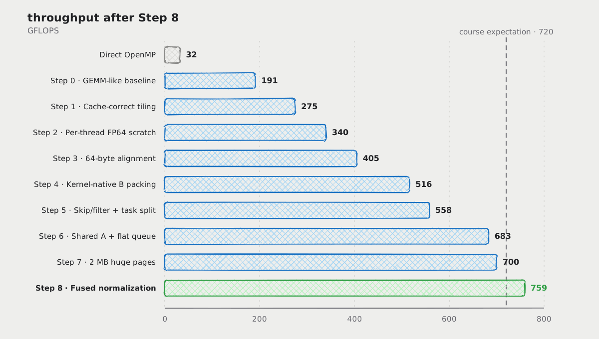
The course expectation for this benchmark is about 720 GFLOPS. The score
counts two useful operations per multiply-accumulate in the requested lower
triangle, while timing the complete call, including normalization, packing,
scheduling, and result conversion.
What can this machine achieve theoretically, and what can optimized software reach in practice?
The theoretical limit is the
compute side of the roofline model.
One AVX-512 register holds eight doubles, each core can issue two vector FMAs
per cycle,
and each FMA performs a multiply and an add. Using the ~3.35 GHz effective
clock assumed in the benchmark notes gives:
18 doubles × 2 operations × 2 FMA ports × 10 cores × 3.35 GHz
2≈ 1,072 GFLOPS
This 1,072 GFLOPS figure is an ideal compute roof: every core executes
useful, full-width FMAs every cycle, with no time spent on anything else.
For a practical roof, Intel oneMKL is a useful reference: it is one of the
most heavily optimized CPU math libraries used in HPC. Its
DGEMM has been reported at about 890 GFLOPS
on the same Xeon W-2255, roughly 83% of the theoretical roof. My complete
correlation pipeline reaches 759 GFLOPS, or 71%. The comparison is not
quite apples-to-apples: oneMKL measures dense matrix multiplication, while my
timing also includes normalization, packing, triangular scheduling, edge
handling, and conversion to the fp32 result.
| Version | Wall-clock | Useful ops/s | % of compute roof |
|---|---|---|---|
| Naive direct implementation (multithreaded) | ~22.6 s | ~32 GFLOPS | ~3% |
| Course expectation | — | ~720 GFLOPS | ~67% |
| Final kernel | ~0.96 s | ~759 GFLOPS | ~71% |
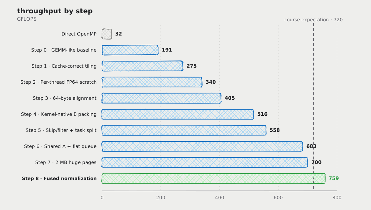
The sections below are implementation lessons, not a cumulative timeline. Each one gives its own score: a measured win, a measured rejection, the score of a final configuration, or an explicit note that the change was not isolated.
Step 0: From direct loops to a GEMM-like baseline Link to heading
I started with the most direct multithreaded solution: normalize every row,
use an OpenMP loop over i, and compute every i, j pair with a plain dot
product.
 1void correlate(int ny, int nx, const float* data, float* result) {
 2    std::vector<double> normalized(ny * nx);
 3
 4    // normalization-and-scale (omitted here)
 5
 6    #pragma omp parallel for schedule(dynamic, 1)
 7    for (int i = 0; i < ny; ++i) {
 8        const double* row_i = normalized.data() + i * nx;
 9        for (int j = 0; j < i; ++j) {
10            const double* row_j = normalized.data() + j * nx;
11            double correlation = 0.0;
12            for (int x = 0; x < nx; ++x) {
13                correlation += row_i[x] * row_j[x];
14            }
15            result[i + j * ny] = static_cast<float>(correlation);
16        }
17        result[i + i * ny] = 1.0f;
18    }
19}
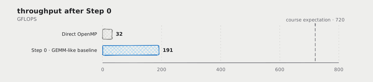
It kept the machine busy — 19.8 hardware threads on average from 20 available — but had no cache blocking, packing, or explicit SIMD.
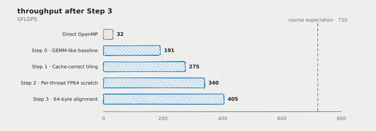
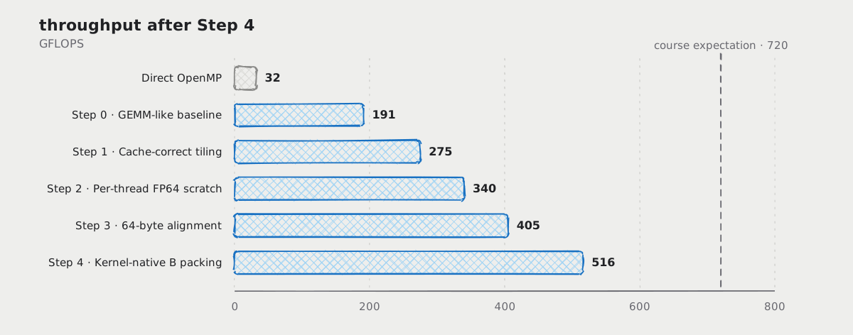
First score. That version took about 22.6 s, or only 32 GFLOPS.
Adding threads was not enough; each dot product still walked complete rows
independently, without organizing their reuse around cache-sized blocks.
After normalization, the same computation can be written as a matrix multiplication:
1A[i,k] = normalized input[i,k]
2B[k,j] = A[j,k]
3C[i,j] = sum_k A[i,k] * B[k,j]
Here B is the logical transpose of A; it does not need to exist as a
separate input matrix.
I then dug into GEMM papers and existing implementations and followed the usual playbook: tile for the caches, pack A and B, run the inner loop in a small microkernel, spread tiles across threads with OpenMP, and write the fp64 arithmetic with AVX-512.
Baseline score. That brought the time down to 3.815 s, or
191 GFLOPS — almost six times faster. On paper, most of the pieces were now
present, but most of the available arithmetic throughput was still unused.
Step 1: Cache-correct macro-tiling tuning Link to heading
In GEMM notation, A is M×K, B is K×N, and C is M×N. For this
correlation task, M = N = ny are the result dimensions and K = nx is the
dot-product length. Accordingly, blockM and blockN tile the output matrix,
while blockK splits each dot product into cache-sized pieces.
At 191 GFLOPS, I got stuck. I changed block dimensions, tried different
kernel sizes, and measured the same code over and over. A few combinations
moved the timing slightly, but none explained why a packed AVX-512 kernel was
still so far from the machine’s potential.
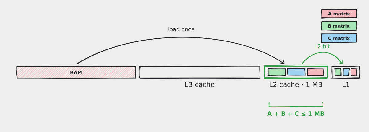
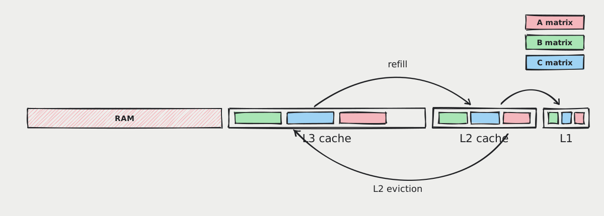
A careful review found the real problem: the L2 cache constant was wrong. The tiling code assumed 4 MB per core, while the target Xeon has only 1 MB. This constant controls the macro-tile, which has to hold packed A, packed B, and a working slice of C.
Ideally — the macro-tile fits in L2:
- An A micro-panel stays cached while it is used against many B panels.
- B panels stay cached long enough to be reused for the next group of A rows.
- The C macro-tile stays cached between successive
blockKiterations.
In my case — the macro-tile was too large:
With an oversized macro-tile, accesses to later portions of A, B, and C evicted earlier portions before reuse. As a result, the same data moved through the cache hierarchy repeatedly.
The fix:
A rough capacity estimate for three square fp64 tiles is
3 × side² × sizeof(double) ≤ L2_size. With a 1 MiB L2 cache, the ceiling is
about 209 elements before alignment and scheduling adjustments.
Many GEMM examples hard-code blockM, blockN, and blockK for one machine
and problem size. In Tencent’s
ncnn library, I found a heuristic that
selects them automatically from the cache size, microkernel
shape, matrix dimensions, and thread count.
Its logic is roughly:
1side   = sqrt(L2_size / (3 * sizeof(double)))
2blockM = round_to_microkernel_rows(side)
3blockN = round_to_simd_width(side)
4blockK = round_to_simd_width(side)
5rebalance_for(M, N, K, thread_count)
For example, for a 24×8 kernel, that means rounding blockM to a multiple
of 24 and blockN and blockK to multiples of eight. The heuristic also
avoids tiny tail tiles. If K fits in one block, it spends more of the cache budget on M
and N; it adjusts M for the thread count so there are enough row tiles to keep
the cores busy.
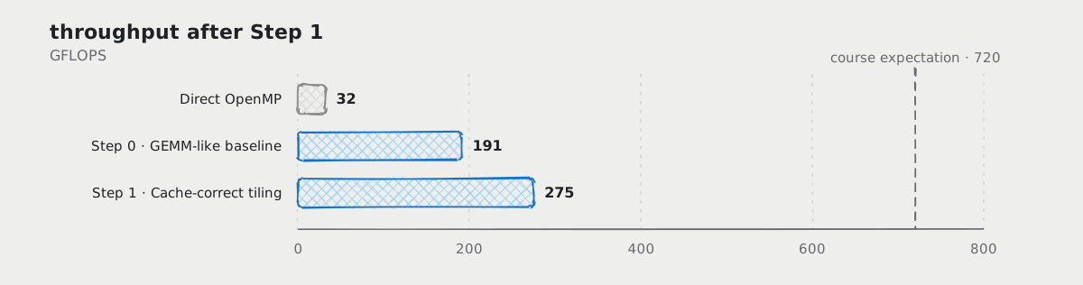
Score. Fixing that one cache-size assumption, with no other code change,
moved the benchmark to 2.651 s / 275 GFLOPS.
Step 2: Store partial sums Link to heading
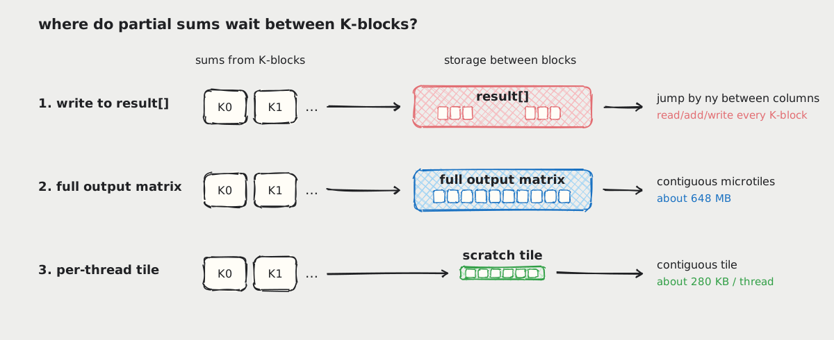
The microkernel updates a compact 24×8 tile one K-block at a time. But
result[] stores the whole matrix, with the next output column ny elements
away. This layout mismatch made the destination for partial sums important.
Write straight to result[]. Each K-block would read the previous sums
from the large result matrix, add its new sums, and write them back. Moving
between columns would jump by ny elements. That puts repeated, scattered
read-modify-write traffic in the hot loop.
Use a full output matrix. The next version kept a global c_output
arranged in contiguous microtiles, then traversed it to fill result[] in
one final pass. The kernel could update nearby values, but the extra matrix
used about 648 MB at 9000×9000 and required a separate full-matrix pass.
Keep one scratch tile per thread. The final design keeps only the
current macro-tile in a per-thread c_block. Each K-block updates this
compact tile; when the tile is complete, the code converts and writes its
values to result[] once. Each tile is about 280 KB, so temporary storage
grows with the thread count instead of ny².
Three storage choices for partial sums between K-blocks.
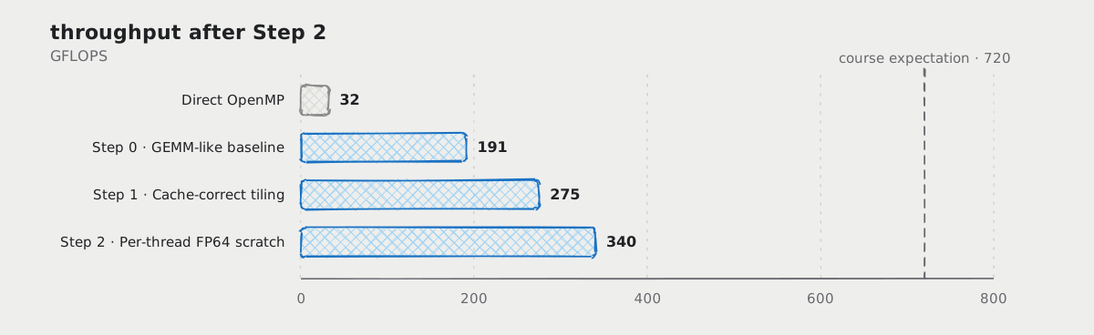
Score. Removing the full output matrix and exporting each finished
scratch tile directly moved the benchmark to 2.142 s / 340 GFLOPS.
Step 3: Alignment is part of the layout Link to heading
Initially, my packed buffers were ordinary vectors:
1std::vector<double> a_blocks(a_count);
2std::vector<double> b_blocks(b_count);
3std::vector<double> c_blocks(c_count);
They are contiguous, so at first this looked fine. But std::vector<double>
only guarantees alignment suitable for a double; it does not guarantee the
64-byte alignment required by an aligned AVX-512 load or store. Sergey Slotin
has a good overview of memory alignment and its performance effects.
I replaced them with explicitly aligned allocations:
1aligned_array<double> a_blocks(a_count, 64);
2aligned_array<double> b_blocks(b_count, 64);
3aligned_array<double> c_blocks(c_count, 64);
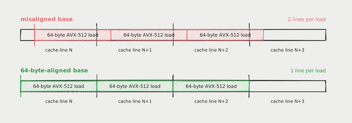
Aligning the base pointer is only half of the job. Every panel stride and microtile offset
must also be a multiple of eight doubles, so that every address handed to _mm512_load_pd stays 64-byte
aligned. In this layout the offsets were already multiples of 64 bytes, which
is exactly what made the base pointer so expensive: a 512-bit load is one
full cache line, so a misaligned base made every A and C transfer straddle
two lines — not occasionally, but every single time — and no later panel
could recover the alignment.
Aligned versus misaligned loads against a 64-byte cache line.
Score. Explicitly aligning the packed buffers and switching the guaranteed
aligned hot paths from loadu/storeu to load/store moved the benchmark to
1.803 s / 405 GFLOPS.
Step 4: Pack for microkernel Link to heading
Before looking at the packing layout, here is the work of one 24×8
microkernel. Each SIMD vector has 8 lanes, one for each output row in its
group. The 3×8 array therefore holds 24 vectors of partial sums:
 1# acc[row_group][column] is one 8-lane SIMD vector.
 2acc[3][8] = load_or_zero(scratch_microtile)
 3
 4for k in current K-block:
 5    a0, a1, a2 = load 24 packed A values at k
 6    for column in 0..7:
 7        b = broadcast packed B value at (k, column)
 8        acc[0][column] += a0 * b
 9        acc[1][column] += a1 * b
10        acc[2][column] += a2 * b
11
12store acc in scratch_microtile
One vector FMA multiplies 8 A values by a broadcast B scalar and adds them
to one accumulator register. Repeating this for 3 A vectors and 8 B scalars
updates the full 24×8 tile.
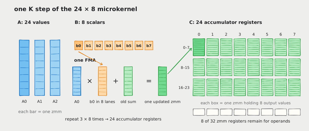
Those 24 accumulators occupy 24 of the machine’s 32 vector registers, leaving room for operands without spilling the partial sums to memory.
The first K-block starts the sums at zero; later K-blocks load the sums left in the scratch tile.
The microkernel works on 8 B columns at a time. After reading those 8 values at one K position, it needs the same 8 columns at the next K position. My first packer arranged B by K position instead:
1packed[k * max_jj + row] = input[row * nx + k]; // B[k, row] = input[row, k]
Here max_jj is the width of the packed B macro-panel. The packer stores all
its columns for k=0, then all its columns for k=1, and so on.
The first packer turns each input column at one K position into a contiguous row of packed B.
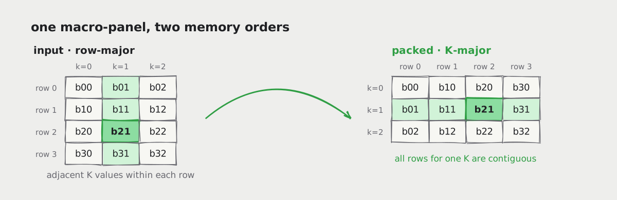
That layout makes each full K slice contiguous. But a microkernel uses only 8
values from that slice. It keeps partial sums for those 8 output columns in
registers; other columns are handled by other microkernel calls. With pB at
the first of those 8 values, the next group is max_jj doubles away:
1const vec b0      = _mm512_set1_pd(pB[0]);      // k=0, first column → all lanes
2const vec b0_next = _mm512_set1_pd(pB[max_jj]); // k=1, same column → all lanes
3pB += 2 * max_jj; // move past two K positions
The main problem was the runtime max_jj stride: the compiler could not
fold B addresses into fixed offsets. It kept B offsets live in integer
registers and emitted extra address arithmetic, increasing register pressure
in the microkernel. With a wide panel, successive K reads also jumped past
values used by other microkernels.
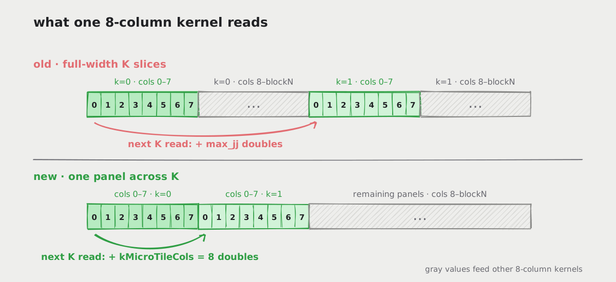
I repacked B so each 8-column panel stays together across K: its values for
k=0 are followed immediately by its values for k=1. After all K positions
for that panel, the packer starts the next 8-column panel. Compared with the
old k * max_jj + row index, the new destination is:
1panel = row / 8
2lane = row % 8
3packed[panel * max_kk * 8 + k * 8 + lane] = input[row * nx + k]
Here max_kk is the number of K positions in the current block. The kernel
can now use a fixed stride:
1constexpr int kMicroTileCols = 8; // B values per K position
2const vec b0      = _mm512_set1_pd(pB[0]);              // k=0, first column → all lanes
3const vec b0_next = _mm512_set1_pd(pB[kMicroTileCols]); // k=1, same column → all lanes
4pB += 2 * kMicroTileCols; // move past two K positions
The kernel still processes the same 8 B columns at each K position, but its
next read is always 8 doubles away instead of max_jj doubles away.
Strided packed B versus contiguous 8-column panels.
Score. Repacking B moved the benchmark to about 516 GFLOPS.
Step 5: Handle diagonal tiles Link to heading
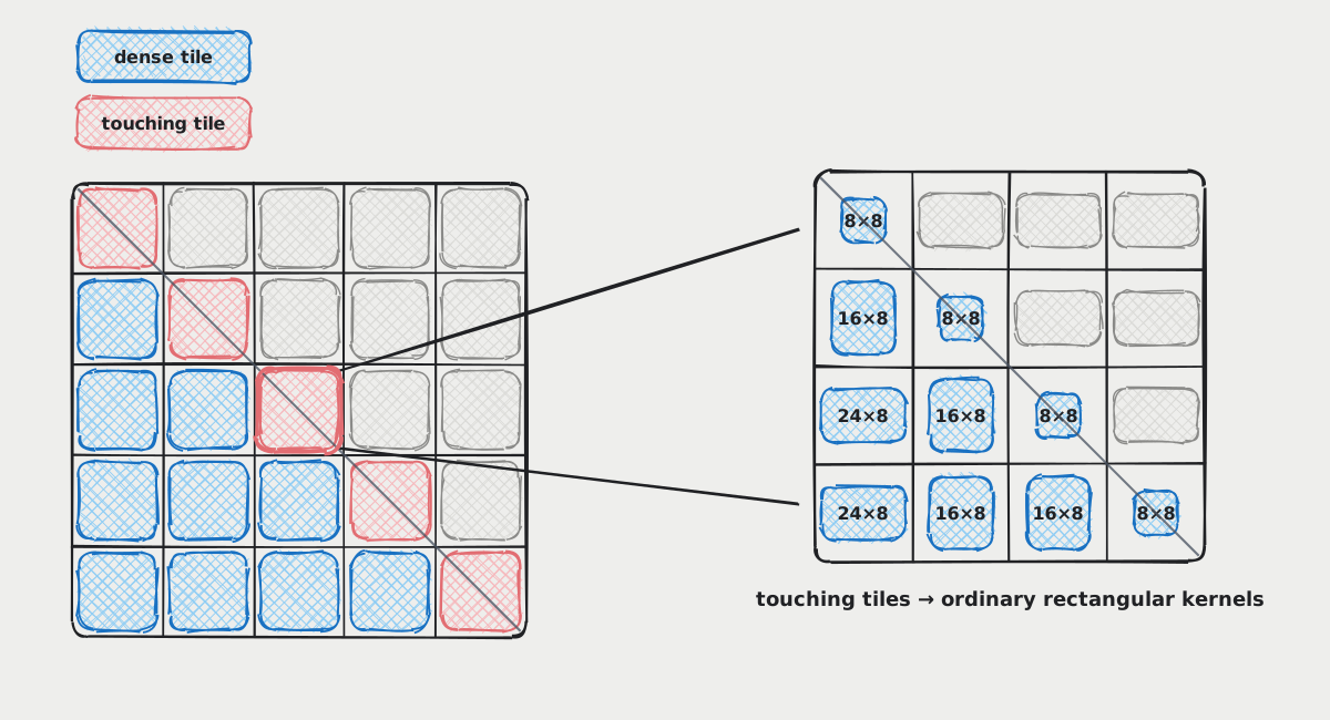
A tile crossing i == j contains three kinds of cells: useful ones, diagonal
ones, and cells above the diagonal that will never be returned. The tempting
move is to teach the kernel about that boundary.
Checking the diagonal inside the main loop added a branch at every K step and slowed it down. Masked SIMD instructions did not help either.
The faster version runs two paths in separate OpenMP phases:
dense_tiles: Fully below the diagonal; use24×8.touching_tiles: Cross the diagonal; choose24×8,16×8, or8×8according to how much of the tile lies in the lower triangle.
Skipped, fully computed, and partially exported diagonal tiles.
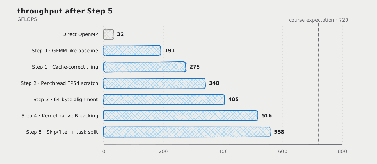
Score. Together, the changes moved the benchmark to 1.308 s / 558 GFLOPS.
Step 6: Partition work between threads Link to heading
Step 5 improved thread utilization, but some threads still finished earlier than others. In a full matrix, equal row ranges contain similar amounts of work. In the lower triangle, they do not. To keep the threads busy, I needed to give each one a similar amount of work.
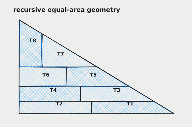
Following Jonathan Lawrence Peyton’s master’s thesis, Programming Dense Linear Algebra Kernels on Vectorized Architectures, I tried a $t_r \times t_c$ partition: $t_r$ row bands, each split into $t_c$ equal-area thread regions. In the continuous-area model, let $n$ be the side of the remaining triangle and $r_1$ the height of the next band. Giving that band $1/t_r$ of the area determines its height:
$$ nr_1-\frac{r_1^2}{2}=\frac{n^2}{2t_r} \quad\Longrightarrow\quad r_1=n\left(1-\sqrt{1-\frac{1}{t_r}}\right). $$
Within the band, let $c_1$ be the width of the region touching the diagonal. Giving it $1/t_c$ of the band’s area determines that width:
$$ c_1r_1-\frac{r_1^2}{2} =\frac{1}{t_c}\left(nr_1-\frac{r_1^2}{2}\right) \quad\Longrightarrow\quad c_1=\frac{\frac{1}{t_c}\left(nr_1-\frac{r_1^2}{2}\right) +\frac{r_1^2}{2}}{r_1}. $$
The rest of the band is rectangular and can be divided evenly. I repeated the construction on the remaining triangle of side $n-r_1$, rounding the cuts to the macro-tile grid in my implementation.
Despite several attempts, my equal-area scheduler was no faster than the previous one, and some versions were slower. I could not make the geometric split work well with the fixed tile grid.
Recursive geometric partitioning of the lower triangle.
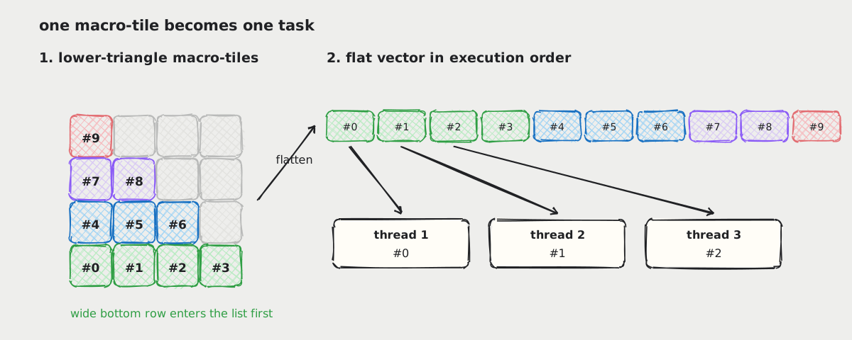
What replaced the geometric regions is much less clever: one flat vector of lower-triangle macro-tiles, sorted by descending rows then ascending columns. Wide row bands start first; within each band, dense tiles come before boundary tiles and B panels stay ordered. Threads pull tasks through a single relaxed atomic counter. No geometry, no regions, no static partition — just a queue.
The same work flattened into a shared queue.
But one problem remained: different threads repeatedly packed the same A panels. I used the same approach as for B: prepack A once into a shared, read-only buffer. This keeps more packed data in memory, but removes the duplicate work and lets any thread process any task.
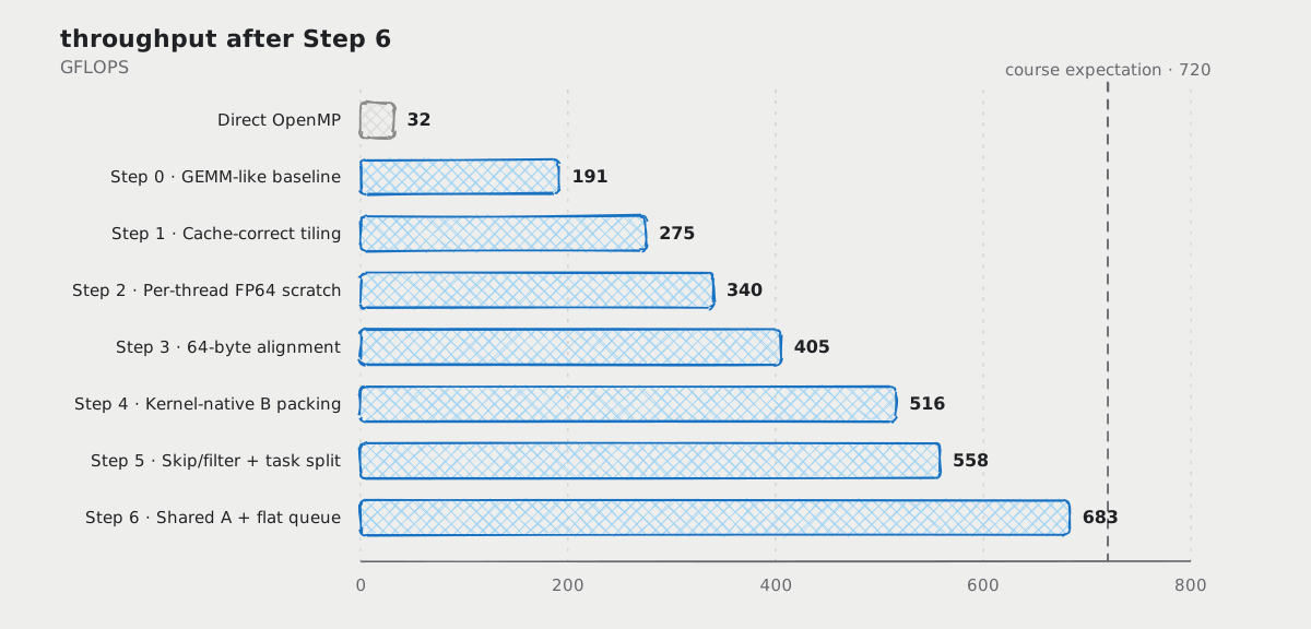
Score. Global A packing plus the flat queue moved the benchmark to about
1.064 s / 683 GFLOPS, with 19.0 threads active on average and 20.2 s of
CPU time.
Step 7: Huge memory pages Link to heading
Profiling showed about 299,000 page faults. The prepacked A and B arrays
were large and read repeatedly, so I investigated why the count was so high.
Linux can back memory with 2 MB transparent huge pages
instead of ordinary 4 KB pages. A program cannot demand that page size through madvise, but
MADV_HUGEPAGE lets it tell the kernel that huge pages are desirable for a
range. The kernel still makes the final decision. I tried that hint on every
large allocation:
1::madvise(ptr, bytes, MADV_HUGEPAGE);
If granted, each 2 MB page replaces 512 ordinary pages, so the buffers need
fewer mappings and fewer page faults when first accessed. But the timing did
not improve, and the page-fault counter stayed at about 299,000. I assumed
transparent huge pages were unavailable on the host and moved on.
The missing condition on this allocation path was alignment. madvise made
the range eligible, but the buffers did not receive huge pages until the
allocations themselves were 2 MB-aligned. Their existing 64-byte alignment
was correct for AVX-512 but insufficient here.
1constexpr std::size_t kHugePageAlign = 2 * 1024 * 1024;
2aligned_array<double> a_blocks(count, kHugePageAlign);
One argument and they simply started working.
Same buffers, backed by ordinary pages versus 2 MB huge pages.
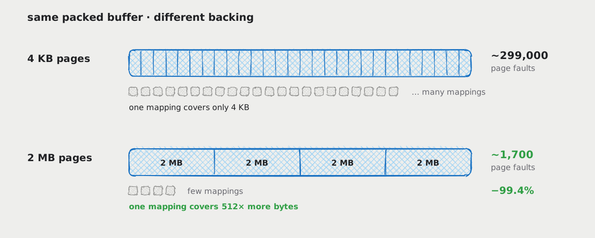
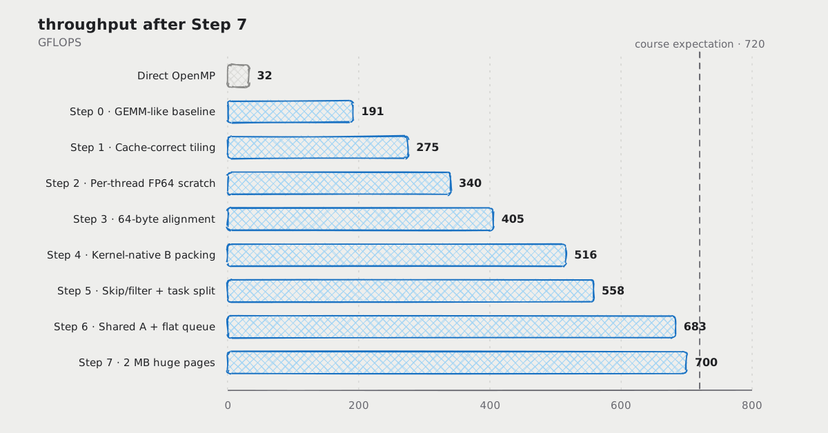
Score. 1.064 s → 1.04 s / ~700 GFLOPS, about +2%. And the counter that
found it: page faults 299,000 → 1,700, a 99.4% drop.
Step 8: Fuse normalization into the packing pass Link to heading
During most of the optimization work, normalization and correlation stayed as two separate stages. First I walked the complete input, normalized every row, and stored a row-major fp64 matrix. The correlation stage then read that matrix again and packed it for the microkernel.
At 9000×9000, the temporary normalized matrix was roughly 650 MB. Every
value was written once by normalization and loaded again by packing before it
reached the kernel.
The fix is almost embarrassing in hindsight: normalizing a row requires only
its mean and its scale. Two small fp64 arrays, one entry per row, are enough.
The packing step then reads each fp32 input value, converts it to fp64,
applies (x - mean[row]) * scale[row], and writes it directly into the
packed layout.
1// Once per row in this packing block, before the loop over k:
2const __m512d mean_v = _mm512_set1_pd(means[i]);   // broadcast scalar into 8 lanes
3const __m512d scale_v = _mm512_set1_pd(scales[i]); // broadcast scalar into 8 lanes
4
5// For each chunk of 8 input values in row i:
6const __m256 raw = _mm256_loadu_ps(row_ptr[i] + k); // raw = 8 input values
7const __m512d x = _mm512_cvtps_pd(raw);             // x = fp64(raw)
8const __m512d centered = _mm512_sub_pd(x, mean_v); // x - mean[row]
9v[i] = _mm512_mul_pd(centered, scale_v);           // centered * scale[row]
Normalize-then-pack versus normalization fused into packing.
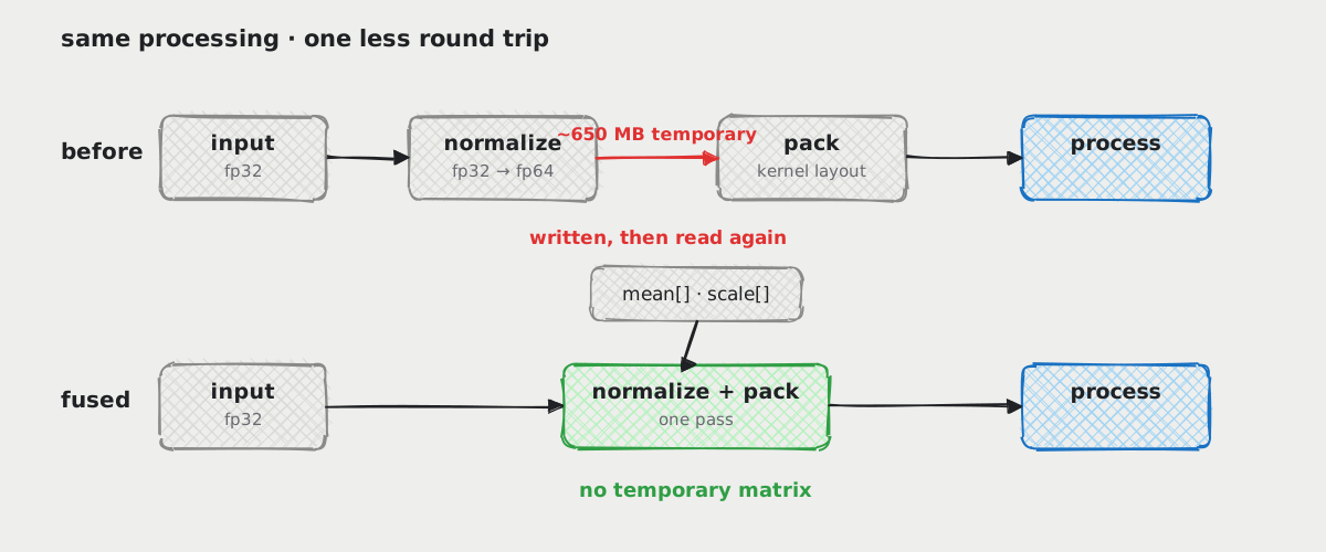
Score. Fusing normalization into packing moved the benchmark to about
0.96 s / 759 GFLOPS. It removed one large allocation and a full write/read
round trip through roughly 650 MB of temporary data.
Final pipeline Link to heading
Here is the full pipeline pseudocode:
 1means, scales = compute_row_statistics(input)
 2packed_A = normalize_and_pack_A(input, means, scales)
 3packed_B = normalize_and_pack_B(input, means, scales)
 4tasks = build_sorted_lower_triangle_tasks()
 5
 6parallel workers:
 7    scratch = one macro-tile per worker
 8    while task = atomic_claim_next(tasks):
 9        for each K-block:
10            for each microtile selected by the dense/diagonal path:
11                A = view(packed_A, microtile.rows, K-block)
12                B = view(packed_B, microtile.columns, K-block)
13                accumulate(A, B, scratch[microtile])
14
15        export cells with row >= column from scratch as fp32
Further reading Link to heading
- The Roofline Model.
- Algorithms for Modern Hardware by Sergey Slotin.
- LAFF-On Programming for High Performance, a course about matrix multiplication optimization.
- Advanced Matrix Multiplication Optimization on Modern Multi-Core Processors by Amanzhol Salykov.
- Fast Multidimensional Matrix Multiplication on CPU from Scratch, by Simon Boehm.
- Programming Dense Linear Algebra Kernels on Vectorized Architectures, a master’s thesis by Jonathan Lawrence Peyton.
- Tencent ncnn, a high-performance neural-network inference framework optimized for mobile platforms.